SOFTWARE ENGINEER

To keep tracking my skills & accomplisments

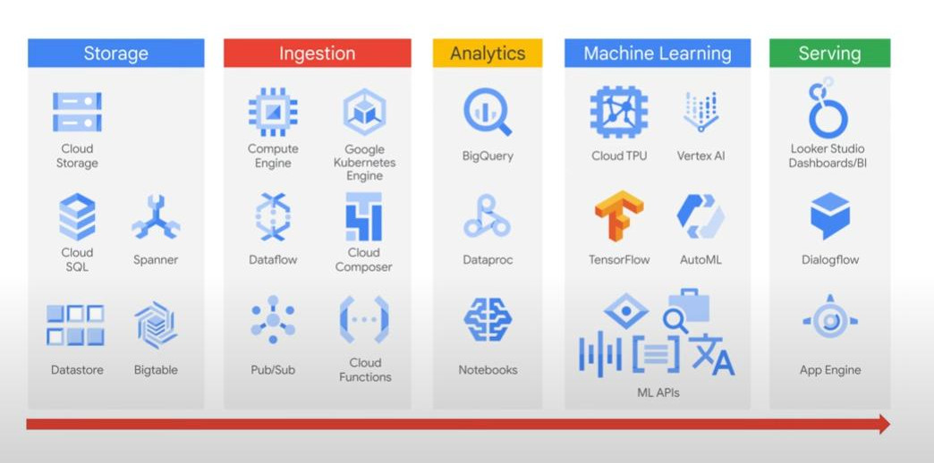
Building, deploying, and operating effective flexible data pipelines for all the stages of data processing is a primary expectation from a pro data engineer.

1. “Migration Task” from existing private data to Google Cloud:

   • Managing and securing data (must comply the regional laws and industry regulations)

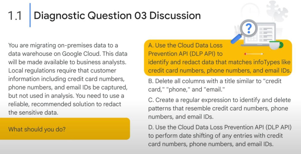
   • Ecrypting and redacting data (like avoid revealing “sensitive data” from being exposed to analysts)

   • “Fined-grained control”: all departments does not need to access to all the data simultaneously. (sensitive information = personal identifiable information - PII = credit card numbers, phone numbers, emails)

   • Key Questions:

   

   

   Key points:

   • 1MB = 8bit => upload speed: 100Mbps (bit) = 100/8 MBps = 12.5 MBps (Byte) => to upload 1TB (~8.4 mByte) we need 23.4 hours ~ 1 day

   • Dataprep: Load the data into it, explore the data, and edit the transformations as needed.

   • Move hundreds of terabytes of data onto Google Cloud: Order a transfer appliance, export the data to it, and ship it to Google. (“gcloud Storage” is just for a small )

   • Cloud Storage: These worker nodes can read the data and also write to it for intermediate storage between processing jobs.

   • Create top level folders for each region, and assign different policies at the folder level.

   • Dataplex: Implement a data mesh with Dataplex and have producers tag data when created.

   • Object retention: Store the data in a Cloud Storage bucket, and specify a retention period. (how long the files should remain without allowing any changes)

   • Cloud Profiler: The code is running slow and you want to further examine the pipeline code to get better visibility of why.

2. Ingesting and processing data:

   • For real-time data, tools are Apache Beam and Dataflow.

   • As the volume of data and scale of processing increases, whether it can make latency, effort and cost to increase linearly, or worse, exponentialy or not.

   • Federated Queries >< normal queries : the difference is the data stored externally and inside Bigquery respectively. Some data is static, whereas others are dynamic. Federated queries allow access of Cloud SQL data directly from BigQuery. This is convenient when the data is changing frequently.

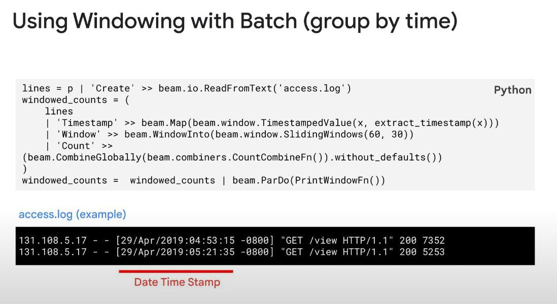
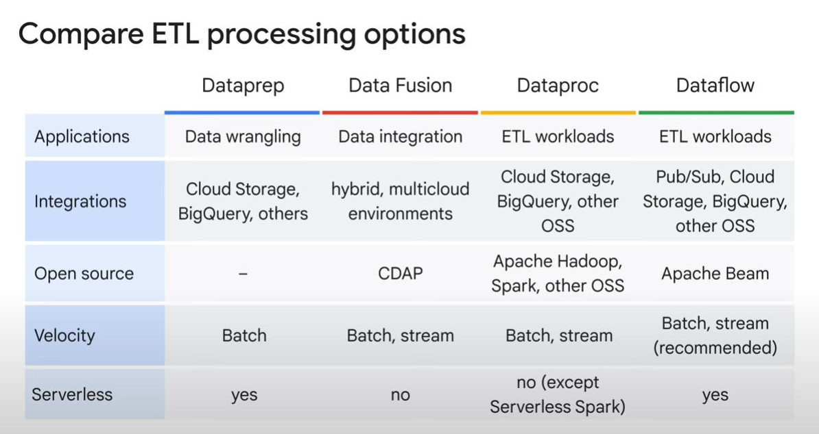
   • Most of the time, the incoming data will be in a raw format and you will need to do complex data processing to transform that data into a suitable form. A Professional Data Engineer should be familiar with multiple tools including Dataproc, Dataflow, Data Fusion, and Dataprep, among others, and use an appropriate tool based on your use case. There are batch data as well as real time streaming data. Streaming data pipelines are significantly more complex than the batch pipelines and data engineer should be familiar with the concepts like windowing, late inputs, and early evaluation.

   • Batch jobs can run for hours and days, Google Cloud has multiple serverless options, including with some Dataproc workloads. Using them can save effort on cluster management.

   • Batch is a fully managed service that schedules, queues, and executes batch processing workloads on Google Cloud. Batch is a managed service that automatically provisions resources to run the batch processing that you configured

   • When data is non-finite but you need intermediate results, windowing helps separate the entire time period into intermediate time periods of processing. Combined with watermarks and triggers, windowing gives the developer the flexibility to control when data processing occurs. A tumbling window (or fixed window in Apache Beam) is fixed duration and non-overlapping.

   • Streaming analytics requires tools that are tuned to continuous processing. On Google Cloud, Pub/Sub, BigQuery, Dataflow, and Datastream are a few of the tools that are recommended for streaming analytics.

   • Cloud Build can be configured to watch for updates in the source repository and trigger a series of steps, as required, to implement a CI/CD pipeline.

3. Storing Data:

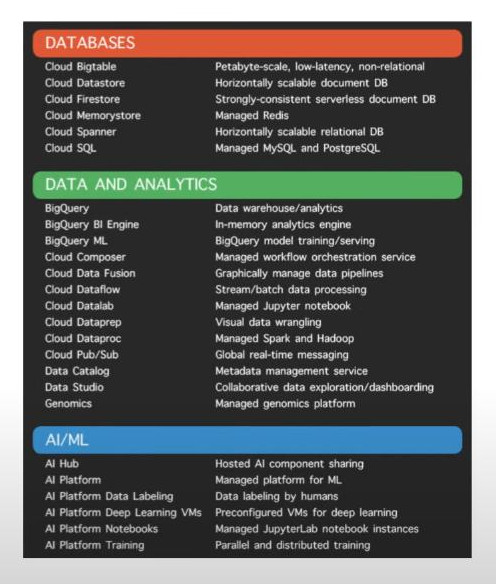
   • GC offers variety of databases: SQL, NoSQL, data lakes, data warehouse, data meshes.

   • Data life cycles must comply with local data privacy rules.

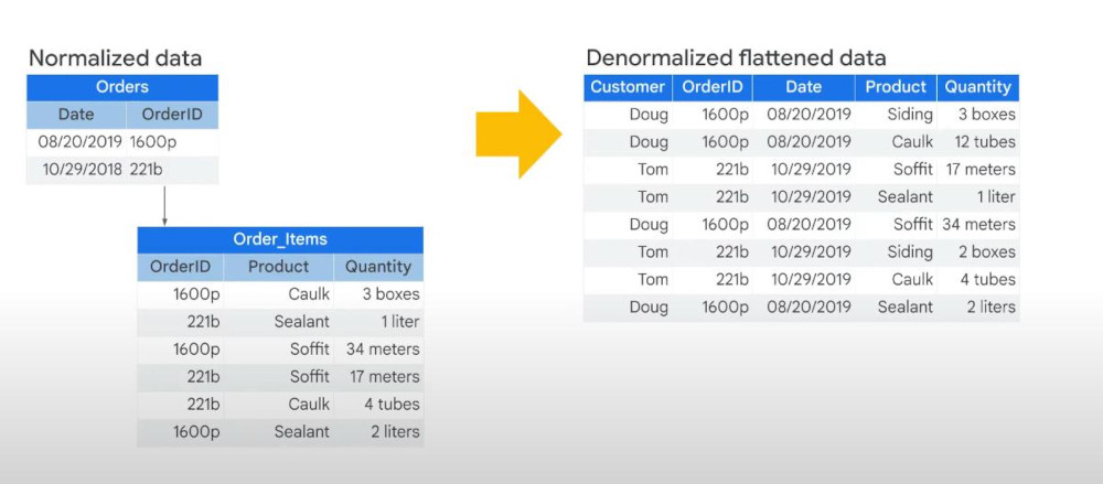
   • Denormalize data >< normalize data: denormalizing data means add more redundant info (un_necessary but easy_to_read columns) into a table to reduce the query complexity.

   • The user has access if either IAM or ACLs grant a permission.

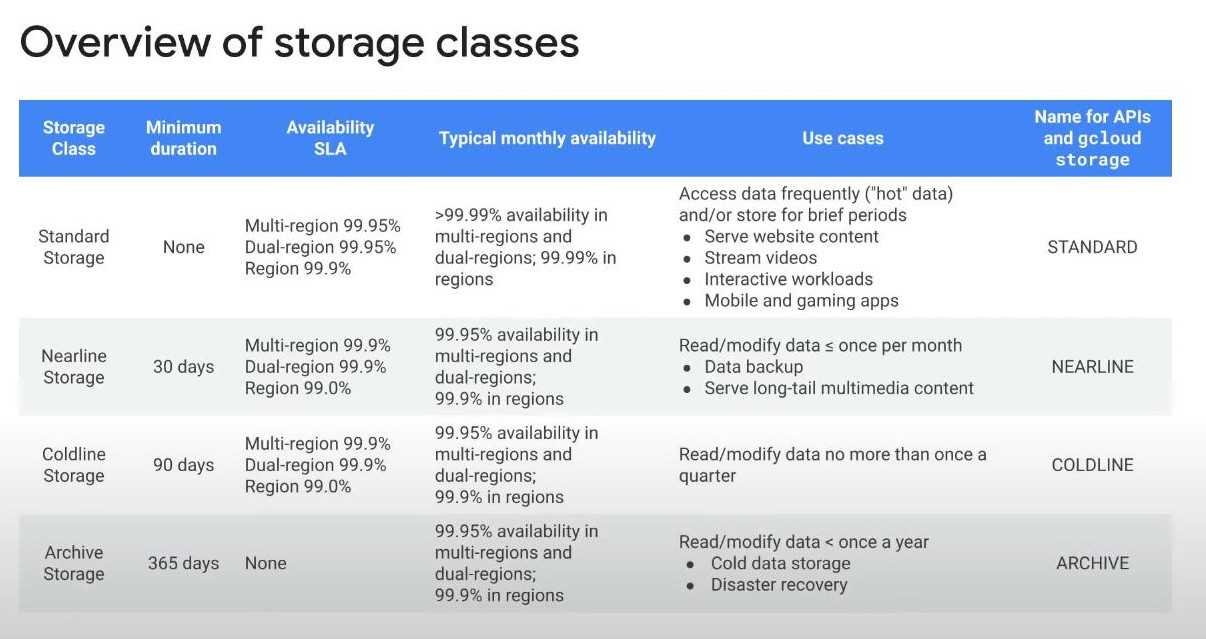
   • What storage class should you choose?
     • Archive (yearly retrieve)
     • Standard (daily fetching)
     • Nearline (monthly)
     • Coldline (quarterly)

4. Preparing & Using data for Analytics:

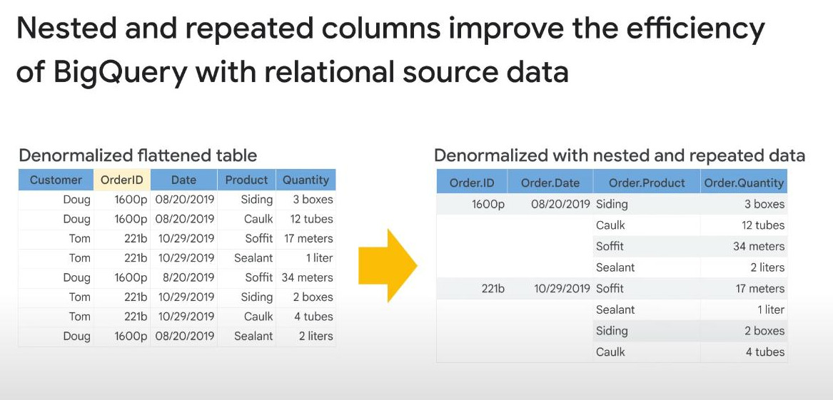
   • The normalized form is suitable for transactional databases, but unsuitable for analytical databases. Joins take time. Collecting related data together with nested and repeated fields can make the data more efficient to read.

   • Views rerun the query each time on the source data; therefore, is not optimal. Materialized views will improve query performance by precomputing and periodically caching query results.

   • A window function in SQL is a powerful feature that performs a calculation across a set of rows that are related to the current row, without collapsing the rows into a single output like aggregate functions typically do.

   • BigQuery performance tuning is a key function that the data engineer needs to perform. You should identify bottlenecks and apply various performance tuning techniques such as partitioning and clustering, batch updates, rewriting queries to filter data as early as possible, avoiding SQL anti-patterns, and other options.

   • BigQuery benefits:

   

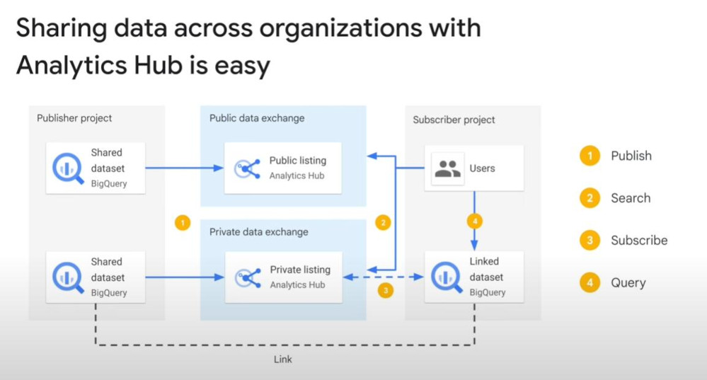
   • Analytics Hub has the built-in options to connect publishers and subscribers with access control and to monetize data access.

   • Machine learning is vital for businesses. However, getting satisfactory results requires fine-tuning the model in different ways. A Professional Data Engineer can improve model performance with techniques such as feature engineering, where you choose the relevant columns and combine them to make the data relevant.

5. Maintaining and Automating Workloads:

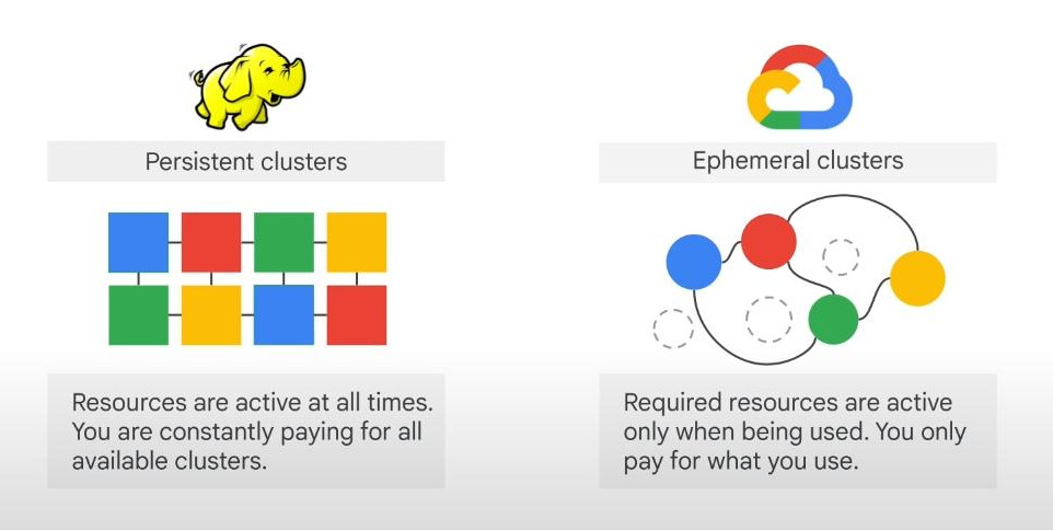
   • Ephemeral clusters: Jobs can use ephemeral clusters to quickly run the job and then deallocate the resources after use. Multiple jobs can be run in parallel without interfering with each other.

   

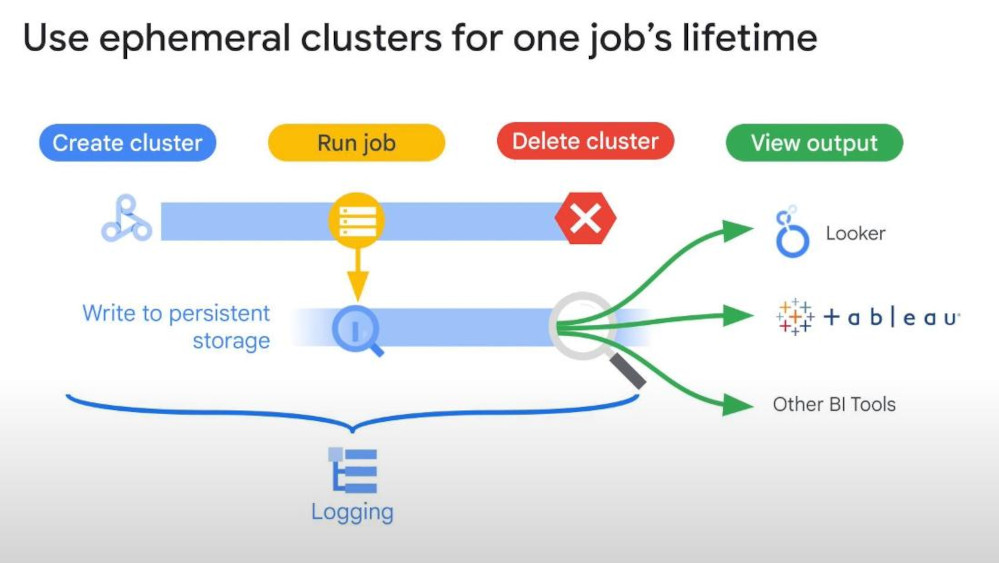
   • Persistent clusters: costs more than ephemeral clusters

   

   • To run repeatable tasks, it is recommended to use atomic tasks that have a single responsibility. Many of these tasks can be combined in sequence to achieve a desired end result.

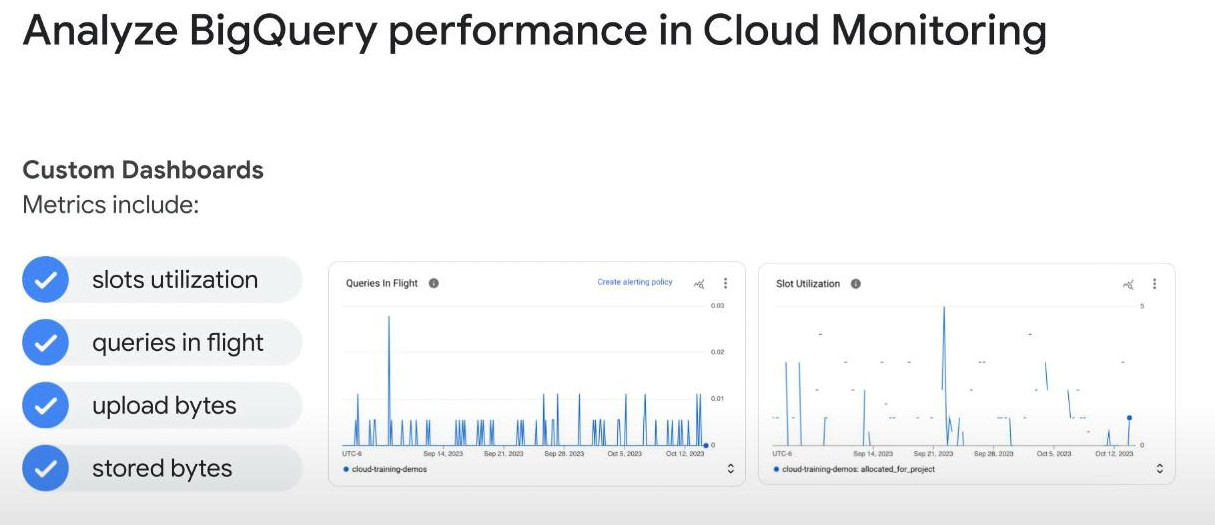
   • Reports on Monday mornings due to which there is heavy utilization of BigQuery => Flex Slots let you reserve BigQuery slots for short durations.

   • Logs: too many concurrent queries for this project_and_region => Run the report generation queries in batch mode.

   • Track and resolve pipeline issues: Set up alerts on Cloud Monitoring based on system lag.

   • Error in the logs: “A hot key HOT_KEY_NAME was detected in…”: => The Dataflow transformations are more performant with an evenly distributed key.

   • Single job clusters are well suited for autoscaling because there won’t be any overlap with scaling of other jobs.

   • Streaming data on Dataflow with Pub/Sub as a source. To plan for disaster recovery and protect against zonal failures: => Take Dataflow snapshots periodically.

   • Get minimal downtime for database: => Configuring high availability on Cloud SQL will automatically switch to the secondary instance when the primary instance goes down, thus reducing downtime for the database’s users.

6. Service APIs in Google Cloud:

   • Types of data: Asynchronous messaging, Unstructured (img, doc, audio) & structured, Relational databases.

   • Data storage options: Cloud storage (unstructured), Spanner, Pub/Sub (messaging), … (Note: BigQuery can store both unstructured and structured data. Cluster in Cloud SQL is up to 64TB for storage and can be scaled if enabled, For BigQuery it is unlimited (charged by amount), for Google Kubernetes Engine is 64TB)

     • Cloud SQL for RDBMS (PostgreSQL, MySQL with high-frequency writes): auto-encryption, 64TB storage capacity, 60-000 IPOS (Input-Output per Second), Autoscale, Auto-backup. It is record-based (row-based) storage, whereas BigQuery is column-based storage. Row-based storage is suitable for transactional workloads, 1 row/transaction, column-based storage is suitable for analytical workloads, where aggregations, filtering or grouping are performed on a large dataset. It is up to 7 backups, 64 processor cores, 100GB RAM.

     • Firestore for NoSQL:

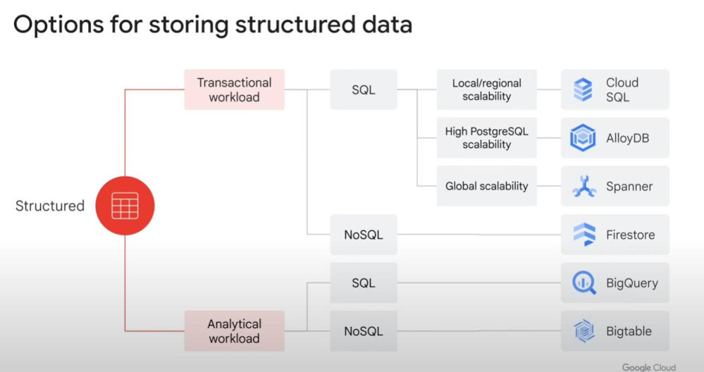
     • For analytic workloads on structured data: we can use BigQuery or Bigtable. A unique feature of BigQuery is that we can create a machine learning model directly inside it with BigQuery-ML. Bigtable is faster and fit for high-throughput millions of rows per seconds (pls check latest throughput).

     • OLTP system (Online Transaction Processing): for transaction system with high-frequency writes.

     • OLAP system (Online Analytical Processing): for analytic system with 20% writes and 80% reads.

     • Failover Replica: like a backup for an instance data in Cloud SQL, located in same region but different zone. It is charged. As outage occurs, Cloud SQK will auto connect to Failover replica and a new Failover replica will be auto-created.

     • Spanner: select Spanner when we require a globally distributed database. Second reason for Spanner is if the database is too big and not fit into one Cloud SQL instance. Third reason for Spanner is when you need horizontal read-write scaling.

     • Note: It’s better to build a pipeline: from customer storage -> Cloud Storage -> BigQuery. If we bypass the Cloud Storage, we can meet internet bottleneck that will make the analytic workloads slower.

   • Data transformation: data can be processed by Dataproc, Dataform, Dataflow. Two main types of data pipeline:

     • Batch pipeline: Dataproc, Dataflow.

     • Real-time analytics: recieve it from Pub/Sub, transformed it using Dataflow or Dataproc, stream it into BigQuery.

   • Dataflow is always the first choice of making a pipeline, but when to use Dataproc or Data Fusion:

     • Dataproc: if we need “reusing Spark pipelines”.
     • Data Fusion: if we need visual pipeline building for non-coding users.

   • Lineage (dòng giống): it’s like metadata of a data (format, qualities, goal-oriented, transformable).

   • Data Catalog (enterprise-level): it needs LABELs (key: value), labels are very useful to filter everything in Google Cloud such as:

     • Billing: With labels attached to any component, we can filter out how much the consumption is for that component?
     • Management: if our project are too big with many datasets, tables. Data Catalog help us to discover or find out the giant data quickly. HOWDY!?

   • Data sink (stored processed data in GC): BigQuery, Dataplex, Bigtable (NoSQL), Analytics Hub. (BigQuery can scan terabytes in seconds and petabytes in minutes).

   • Object Size in Cloud Storage is maximum 5TB.

   • No one size fits all. We have to choose one among various cost-effective storage services:

   

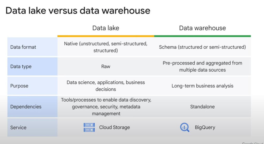
   • Data lakes vs data warehouse:

   

   • Key consideration when you build a data lake:

     • Can your data lakes handle all types of data you have? (fit totally in Cloud Storage bucket?, because if it’s RMDBS data, we have to put in Cloud SQL (managed relational database service) rather than Cloud Storage (Object storage for unstructured data, images, audios).).

     • Can it scale to meet the demand? (when it will run out of disk space? There are 2 types of scaling: horizontal scaling (more nodes, virtual-machines) & vertical scaling (more CPUs,memory, disk space))

     • Does it support high through-put ingestion? (network bandwidth?)

     • Is there fine-grained access control to objects? (Is it enough to get a file as a whole? Cloud Storage is blob storage so we have to think of granuality as storing)

     • Can other tools connect easily? (Cloud Storage is globally accessable, Cloud SQL just for e-commerce, banking apps).

   • Considerations as choosing a data warehouse:

     • Can it serve as a sink for both batch and streaming data pipelines? (Data warehouse is definitely a sink. Is it accurate up to minute for streaming pipeline or is it enough space for a week or just a day?)

     • Can the warehouse scale to meet your needs? (By default, a project is limited to 1000 concurrent-queries (concurrent query-slots) in BigQuery, whereas which is configurable and nearly not limited in Dataproc.).

     • How is the data organized, cataloged, and access controlled? (Who can access and do querying? and Who will pay the querying? Do we need to creat indexes (database), do partitioning or clustering (BigQuery)).

     • What level of maintenance is required by our engineering team? (**)

   • Sharing with security & freshness:

   

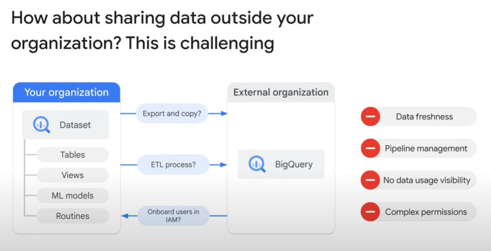
   • Analytics-Hub is very good for sharing across organizations.

   

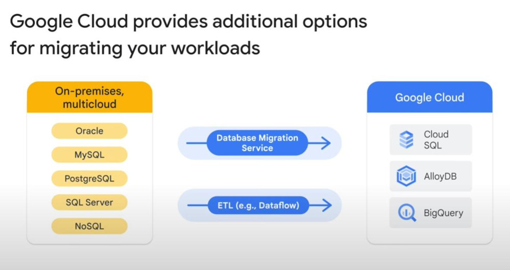
7. Replication & Migration Architecture:

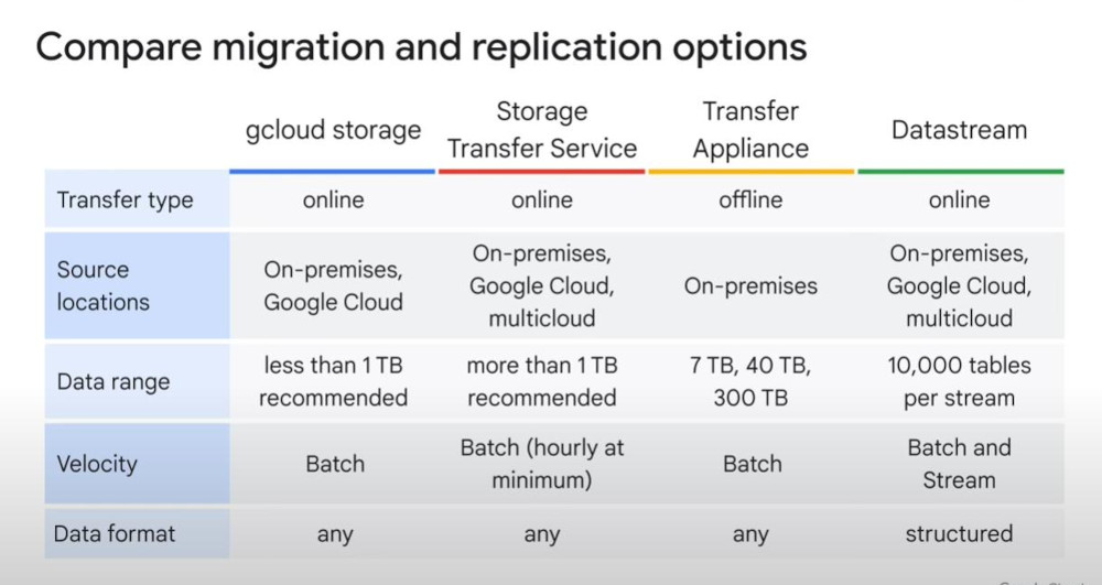
   • Replication & migration: gcloud storage, transfer Applicance, storage transfer services, Datastream.
   • Data could be files system (traditional format like NTFS), Object store (AWS), HDFS (Hadoop), RDBMS (database like Orable, PostgreSQL, MySQL). Each will have proper services:

   

   

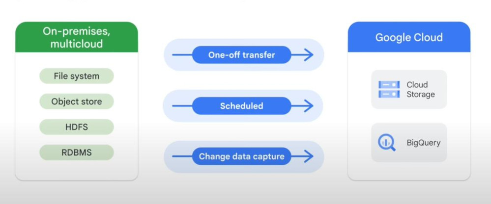
   • Data Size and internet speed (network bandwidth) will lead to which type of migration service.

   

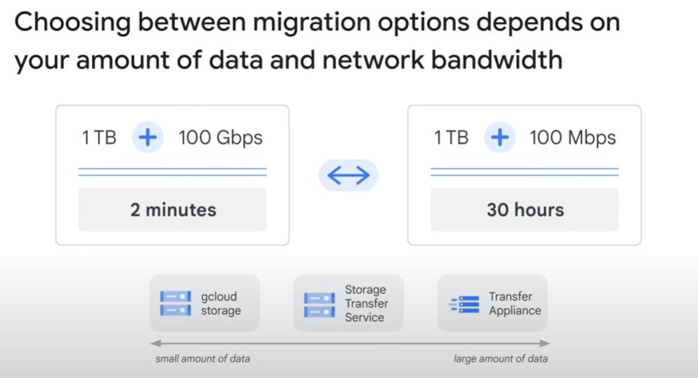
   • gcloud storage: small to medium-sized data with command: _gcloud storage cp _.csv gs://mybucket*.
   • Storage Transfer Service for AWS S3, Azure Blob Storage.
   • Transfer Appliance: for a massive data and limited internet speed, we need a Google-owned hardware as medium storage, copy your data into it, then send it back to Google.
   • Datastream: perfect for RDBMS (Relational DB), can include “data processing” or “normalize data” on-the-way. It can be used with Dataflow templates.

   

   • Datatype of numbers in database: decimals, numeric, and number. Decimal & Numeric is more precise so used for financial app. Number is good to handle a wide range from very small numbers to a very big numbers, so fit for scientific calculations.

   • Metadata: contains context about the data: timestamp, source table, payload (changes),

8. EL - Extract & Load Pipeline Pattern

   • quick because there is not transformation.

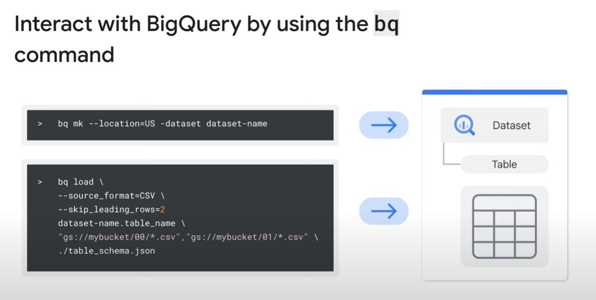
   • EL: extract data (clean or correct) from files on Cloud Storage to BigQuery’s native storage. This pipeline can be triggered by Cloud Composer, Cloud Functions, and scheduled Queries.

   • bq load

   

   • BigLake: allows queries on Cross-cloud object store. So now we have 3 options as analyzing data on Bigquery.

   

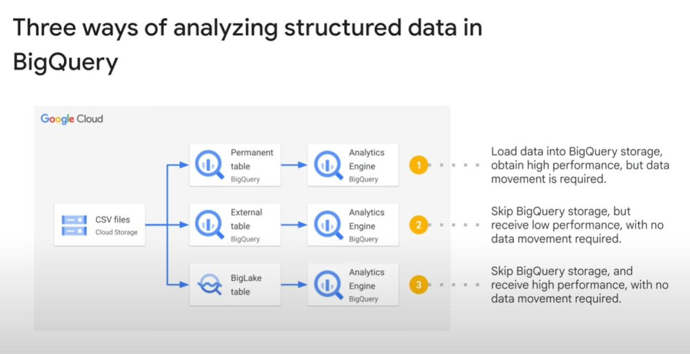
   Warning: “External source of data” will lead to have no cost-estimation feature and caching, BigLake will offer metadata caching within a configurable time, so increase performance.

   

9. ELT - (Extract, Load & Transform):

   • First, it starts with “EL”, so that it is similar to EL, then Transformation happens on the fly using BigQuery Views or stored in new BigQuery Tables. ELT is used when we are not sure about what kind of transformation we will need.

   • Common tools to transform: BigQuery SQL or Dataform SQL-workflow. (Transformation can be scheduled in BigQuery SQL).

   • Besides, we can transform by scripting created in Jupyter Notebook.

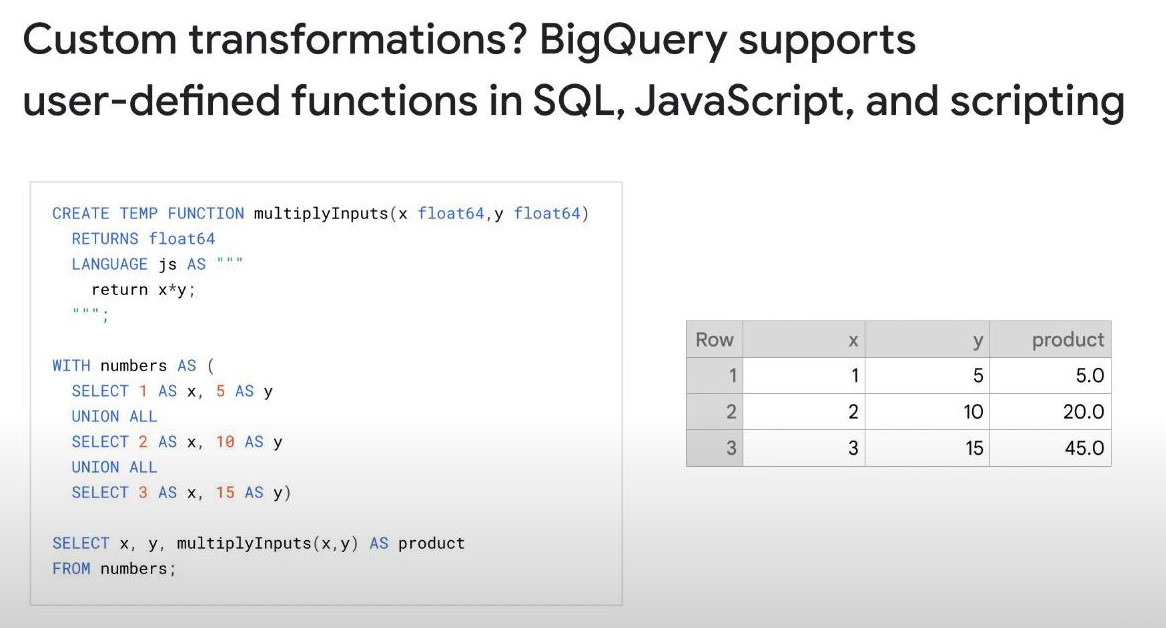
   • BigQuery also support SQL-UDFs (SQL user-defined functions) and JavaScript-UDFs to create functions that can be temporary or persistent.

   • STORED PROCEDURES is SQL statement collections that has benefits of reuseability or flexibility of inputs. BigQuery supports “stored procedures” for Apache Spark, using the command “CREATE PROCEDURE dataset_name.procedure_101” with 3 languages Python, Java, Scala. IT can be stored in Cloud Storage or defined inline in BigQuery SQL.

   • Remote functions or Cloud run functions with more complex programming logic. It can be coded in Python (Cloud Run), then define its connection and use it remotely in BigQuery SQL, similar to UDF. It allows integration of custom logic.

   • Jupyter Notebook + BigQuery DataFrames facilitates data transformation.

   • Matplotlib & seaborn or others for data visualization.

   • BigQuery offers SAVE OR SCHEDULE a query for repeated use. You can save a query, then share it with others. Automation can be enable.

   • DataForm is a serverless framework, used for more complex SQL workflow or ELT pipeline in SQL. It unifies transformaton, assertion and automation . Without DataForm, it can be a time-consuming and error-prone process. Dataform works with BigQuery to manage SQL workflows.

   • Dataform can simplify the ETL pipeline but it requires skill of programming: git, JavaScript, sqlx and even YAML.

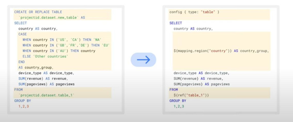
   • Sqlx is a clear framework for organizing SQL code like following:

   

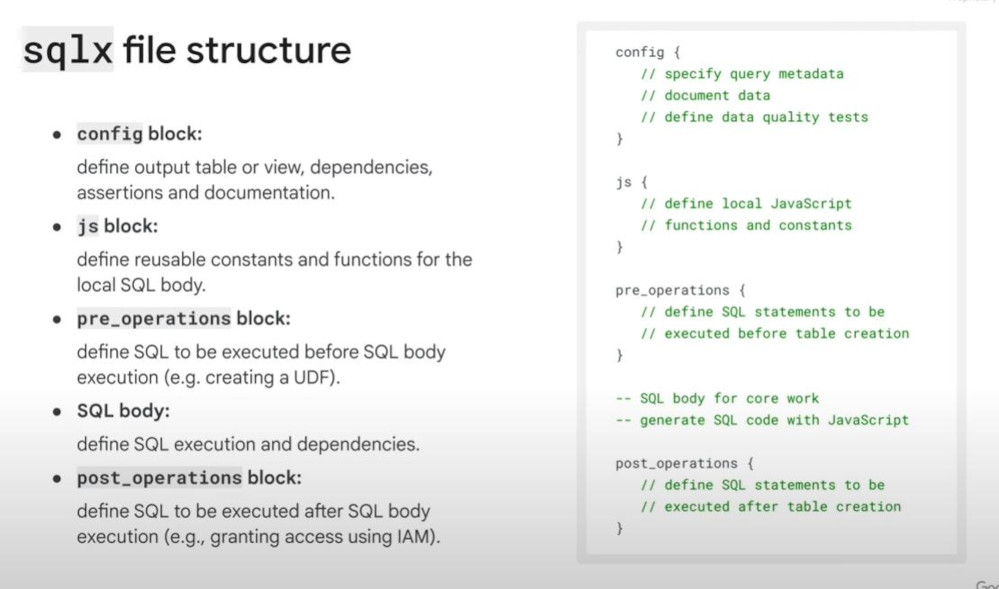
   • An example of SQLX, starting with config {type: …}:

   

   • But why we need ELT, when we have ETL already:
     • When SQL is very complex for Transformation, we should use ETL
     • Streaming is suitable for ELT.
     • For CI/CD or Unit testing requirement, only ELT is fit.

10. ETL - (Extract, Transform & Load):

    • Dataprep is no code solution to build data transformation flow. It can connect various data sources. It provides pre-built functions, allows users to arrange them in a chain, that can be executed with Dataflow. Furthermore, Dataprep even provide visualization of transformation before applying.

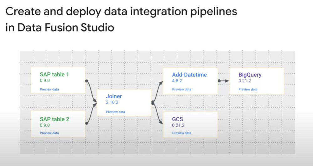
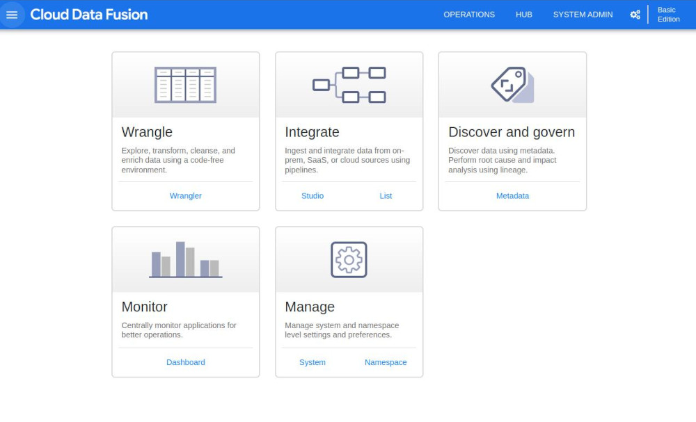
    • Data Fusion is a GUI (graphical) service for enterprise data integration, just drag and drop. It can connect data on both on-premises and cloud.

    

    • DATAPROC allows to run “Apache Hadoop (HDFS)” and “Spark Workloads or Spark jobs” on Google Cloud. Dataproc Serverless for Spark provides an optimized environment designed to easily move existing “Spark workloads” to Google Cloud.

      • Why Hadoop Ecosystem ?: because we need analyze large datasets and Hadoop is a FRAMEWORK that can build a cluster of computers (JVMs) and leverage distributed processing across these computers (parallelism), speeding up the analysis of large datasets. (The computer here is a JVM (Java-Virtual-Machine) because Hadoop runs on the platform of Java.). It includes HDFS and MapReduce, HDFS means “Hadoop Distribution File System”.

      • Apache Spark is also a distributed data processing FRAMEWORK for many large data processing. It is super fast because of “in-memory parallel processing” thanks to RDD (Resilient Distributed Datasets), whereas Hadoop is 100 times slower with “Batch processing due to MapReduce” in theory. Since Hadoop is allocated on Cloud at Dataproc, it becomes naturally fast because of Cloud itself, not because of Hadoop:

        • Auto-Scaling and Elastic Compute Power : Traditional Hadoop runs on a fixed cluster size, meaning you need to provision hardware manually. Dataproc automatically adds more worker nodes when needed and removes them when idle, optimizing costs and performance.

        • High-Speed Storage with Google Cloud Storage : In traditional Hadoop, data is stored in HDFS (issue “I/O bottleneck”), which is tied to the compute nodes. In Dataproc, instead of HDFS, you can use Google Cloud Storage, which is faster, more scalable, and more reliable than HDFS. Plus, it’s separated from compute nodes, so you don’t lose data if a node fails.

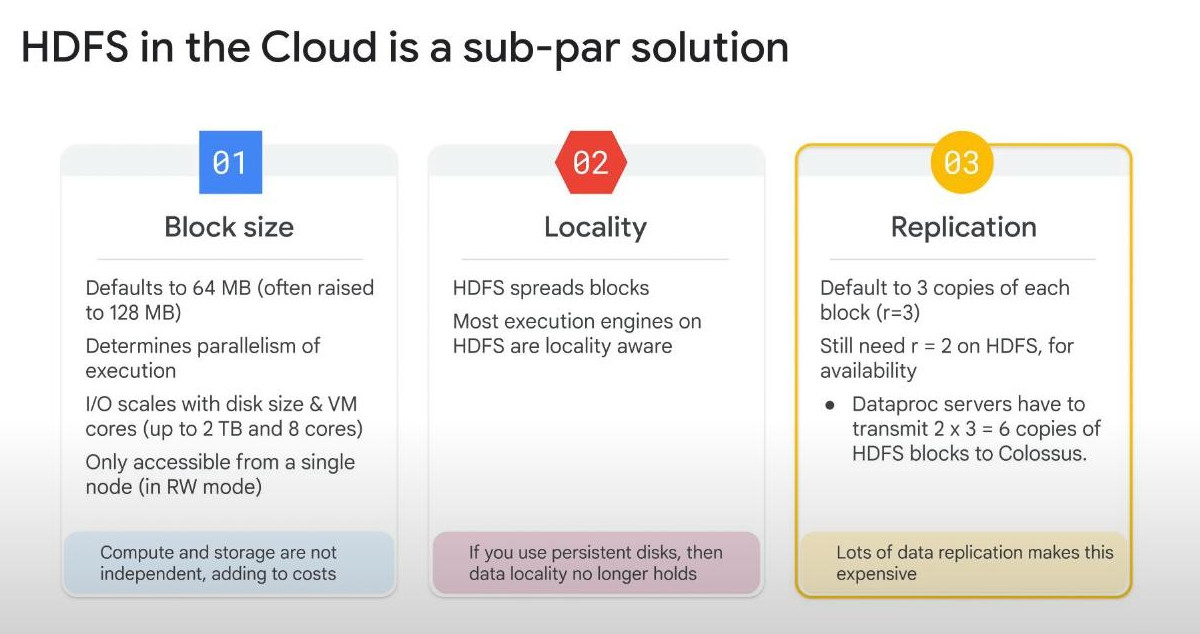
        • Why Cloud Storage instead of HDFS?: In nature, HDFS in Cloud (with persistent disks) is just a subpar (dưới trung bình) solution because it has THREE problems:

        

        • For details:
          • 1. Data Persistence : HDFS exists only while the Dataproc cluster is running. If the cluster is deleted, HDFS data is lost.
          • 2. Scalability : Cloud Storage automatically scales with no storage limits, unlike HDFS, which is limited by the cluster’s worker nodes.
          • 3. Cost Savings : Keeping a Dataproc cluster running costs money. Cloud Storage is cheaper and does not require an active cluster.
          • 4. Integration with BigQuery & AI : Cloud Storage integrates with BigQuery, Vertex AI, Dataflow, and other GCP services. HDFS does not.
          • 5. Disaster Recovery : Cloud Storage replicates data across regions for high availability and fault tolerance. HDFS does not automatically replicate across zones.

      • WARNING: in some cases, local HDFS is still a good options if we are in following cases:

        • There are a lot of metadatas (thousands of partitions and directories and each file sizes are small).

        • Frequently modify HDFS data or rename directories. (Cloud Objects are immutable, so renaming is very exepensive.).

        • Heavily use the APPEND operation on HDFS files.

        • Workloads involve heavy I/O (a lot of WRITE methods).

        • Many Workloads influences latency heavily.

        • Advice: Cloud storage is only good for 2 cases: initial and final sources in the big data pipeline. Medium modified results during computation should be stored in other services. “Dataproc + Cloud Storage” should be used instead of HDFS.

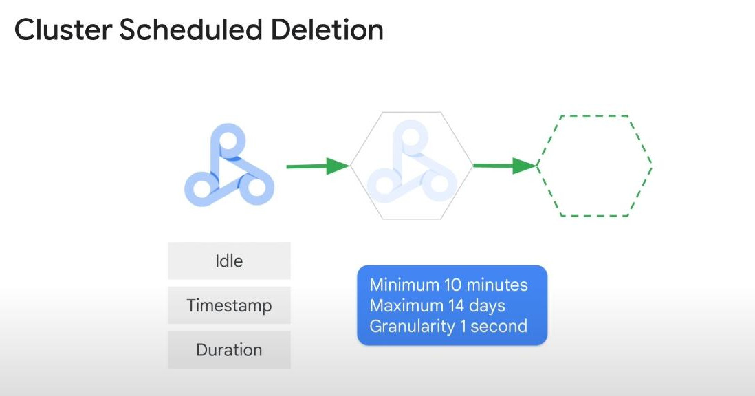
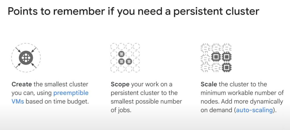
        • In case we need to use “persistent clusters”, we should set “scheduled deletion”:

        

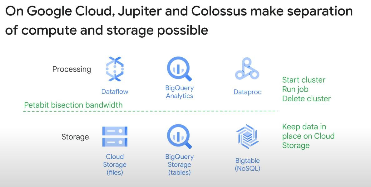
      • Why Dataproc provides both Apache Spark and Hadoop, allowing them to run side by side: HDFS for storage, Hive for SQL queries, Spark for fast in memory processing (train AI models). Moreover, Spark supports more use cases (real-time streaming, ML, SQL, Graph processing). Spark supports Python, R, Scala, Java. This happens because of Jupiter and Colossus.

        • Jupiter is Google’s high-speed, software-defined data center network that relies on a super fast Bisectional Bandwidth (petabit) between 2 groups with a same number of servers.

        • Colossus is Google’s distributed file system that replaces Google File System (GFS) because it stored metadata in a distributed metadata system (metadata stored across multiple nodes), not in a single NameNode like HDFS, so when the metadata grows big (as data grows big), bottleneck issue does not happen with Colossus. It is the backbone of all kinds of Google storage like Cloud storage, Gmail, Drive, Youtube,…

        

      • Why move to Dataproc ?: cheap, no re-configuration or re-development, super-fast (around 90s to turn on/off Dataproc VM), auto-update versions of Spark, Hadoop, Pig, and Hive so we dont need to learn any new things.

      • Tools to interact with Dataproc: Cloud Console, Cloud SDK, Dataproc Rest APIs, multi-options of OSS (open source softwares) to code like Jupyter, Kafka, Spark, Hive, HDFS, Pig…

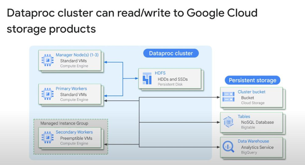
      • A Dataproc Cluster has “Manager nodes (1-3)”, “Primary Workers”, “HDFS”, “Secondary Workers”. When the NATIVE cluster is turned off, we lose everything from it, so we should consider using DIRECTLY cluster on Cloud Storage via HDFS connector, Bigtable for NoSQL DB, BigQuery for Analytics. Code changes very simple from “hdfs//” to “gs//”.

      

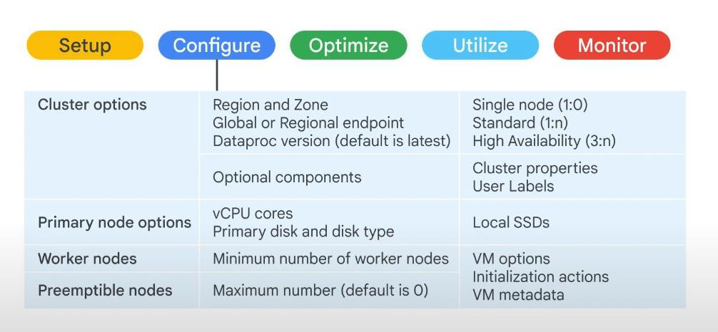
    • Steps or Sequence to use Dataproc:

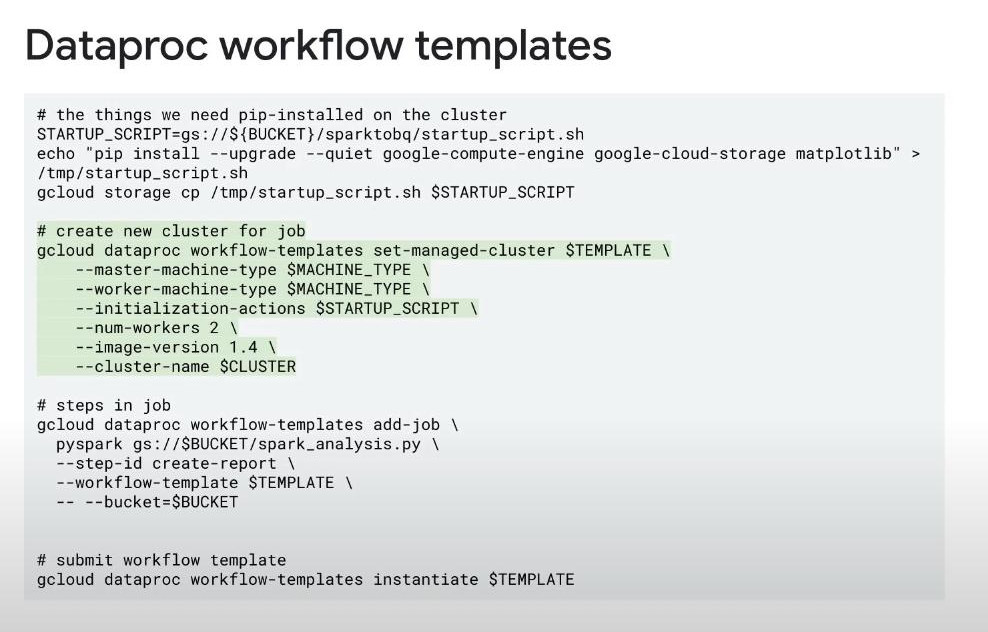
      • Setup: create a cluster with Console, gcloud, YAML, Terraform config, Cloud SDK. We prepare all configuration in the Dataproc Workflow Template (it is a YAML file). We can submit it to the DAG with changeable parameters. Generally, the template contains tasks (create a cluster, selecting existing clusters, submit jobs, deleting a cluster,…) like below:

        

        • The autoscaling will be based on “Hadoop YARN metrics”, adding more worker nodes if the used YARN memory is over 70% (removing idle worker nodes if the used YARN memory is less then 5%.). We can also set min and max number of worker nodes.

      • Config: regional sometimes has lower latency. Primary Node is where HDFS runs (HDFS replication is 2 by default). Pre-emptible nodes including YARN NodeManager don’t run HDFS. Worker nodes is minimum 2 be default.

        • Pre-emptible VMs or pre-emptible nodes - PVMs : a low-cost, short-lived VM that can be stopped anytime by Google Cloud. It reduces the cost 80% compared to regular nodes but we SHOULD NOT use pre-emptible nodes for jobs that are either long (streaming or databases) or unable to accept worker loss (anytime) during running.

      

      • Optimize: Pre-emptible nodes are used and lower cost but notice that they can be pulled from service at any time and within 24h.

        1. Where is the data and where is the cluster? Data region and cluster (VMs) zone should be identical. Set auto-select for cluster zone if possible.

        2. Is your local network traffic being funneled?

        3. How many input files and Hadoop partitions are your trying to deal with? The max number of input files are 10,000 files, try to combine them in larger files if possible. If we have to work with aroud 50,000 partitions, consider to update the parameter “fs.gs.block.size” (the defualt size of a parition is 128MB or 256MB).

        4. Is the size of your persistent disk limiting your throughput?

        5. Did you allocate enough virtual machines (VMs) to your cluster? How many VMs our cluster needs? It’s not easy to answer but we can resize it anytime, so we can run a test.

      • Utilize: jobs can be submitted through the cloud console, the gcloud command, or REST API, workflow templates, Cloud Composer. Don’t use Hadoop Interface to submit jobs because of LACK of metadata. By default, jobs are not restartable but we can create a restartable jobs through the command line or REST API.

        • Split clusters and jobs: isolate dev, staging, and production environments on separate clusters.

        • Points to do if we have to use persistent clusters:

        

      • Monitor: use ‘Cloud Monitor’ or we can set up a dashboard to monitor some alert policy to send notification email.

    • Dataproc Serverless for Spark is a useful API of Google Cloud Engine. It offers batch or session, can connect with other APIs like BigQuery, Cloud Storage. It’s like a virtual machine on GC. “Serverless” means a server that is auto-scaling, fast setup and no cluster management, pay-per-use.

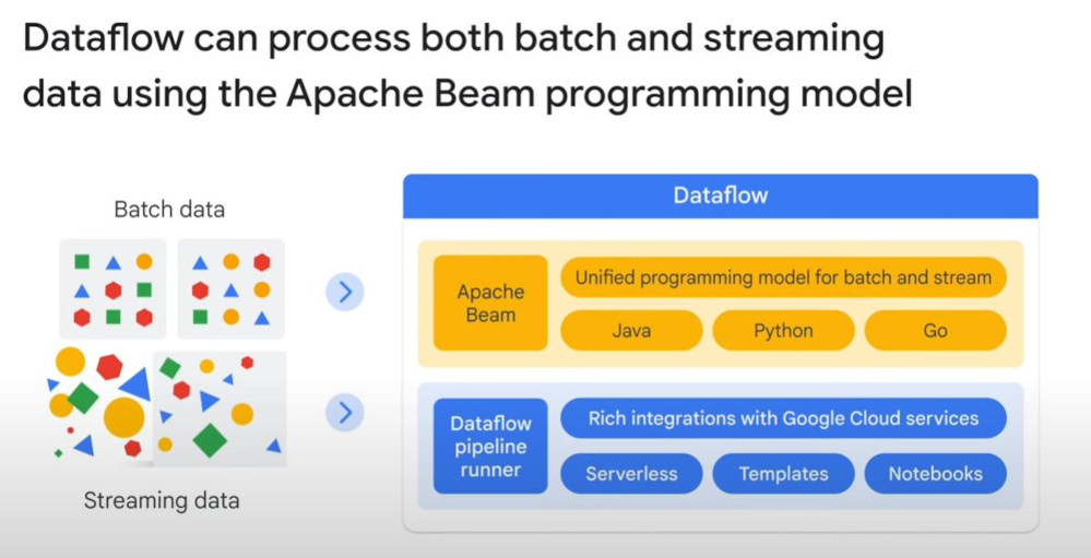
    • DATAFLOW:

      • Batch processing VS streaming data processing: Streaming ETL is almost real-time analytics. “Pub/Sub” is for streaming ETL ingestion. Dataflow can process both “batching and streaming data” using Apache Beam.

      

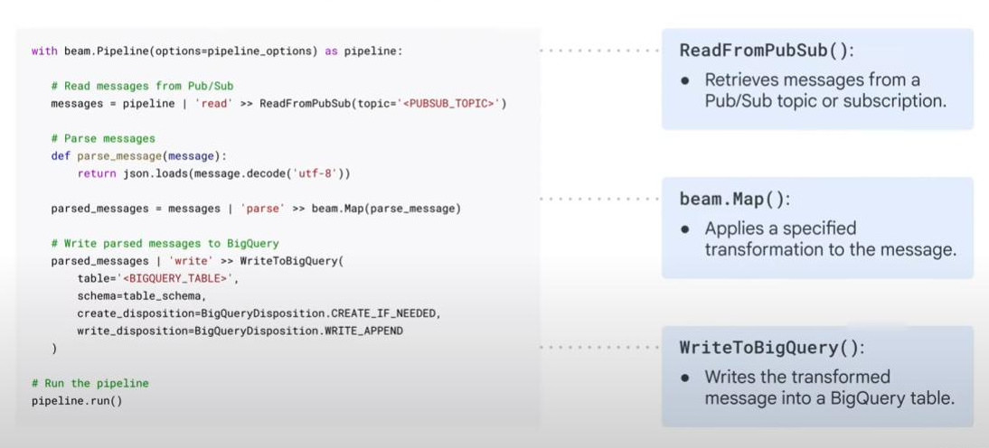
      • Example of Streaming & transforming data from Pub/Sub to BigQuery, using Apache Beam.

      

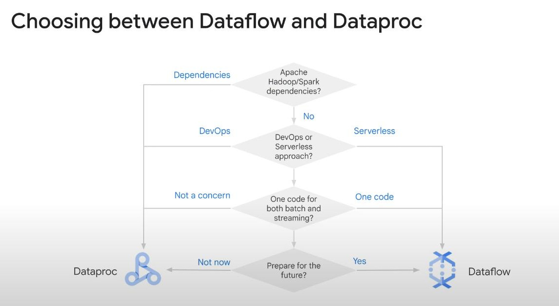
      • How to choose between Dataflow and Dataproc :

      

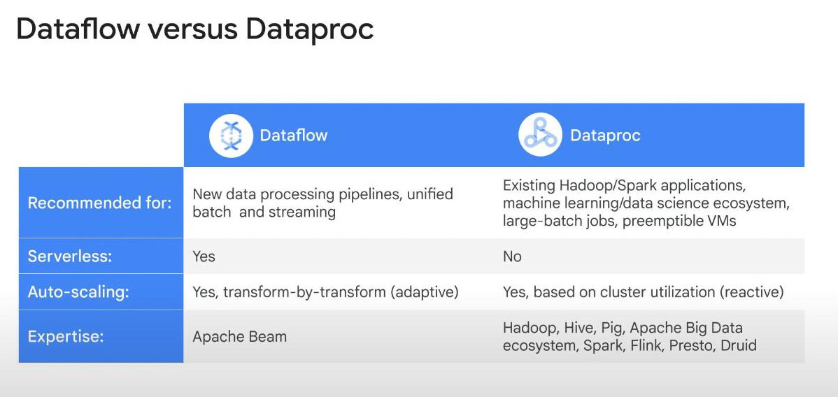
      • At first, dataflow allows using the same code for both batching and streaming.

      

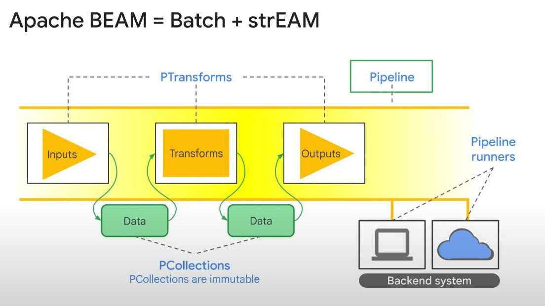
      • Apache Beam in Dataflow: take note that Apache Beam is the core key behind Dataflow. It includes PTransforms, PCollections, Pipeline, Runners:

        • PTransforms : handle inputs, transformation and outputs of the (batch/streaming) data.

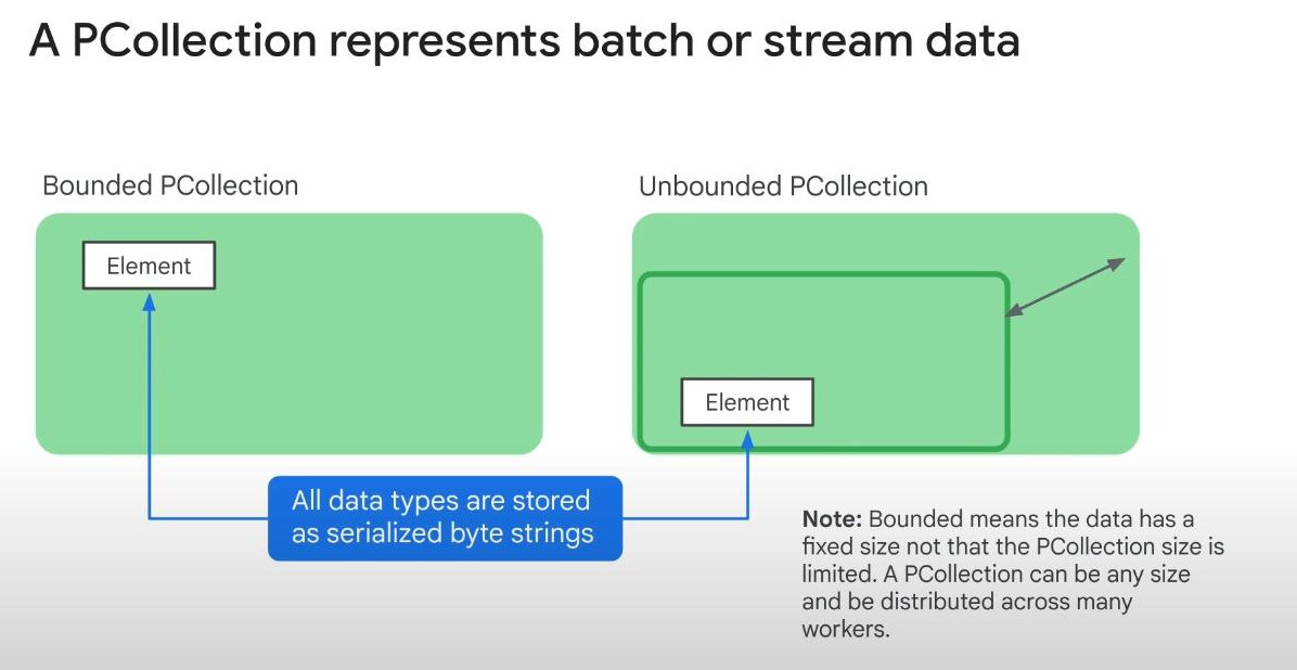
        • PCollections : represents both batch data and streaming data. All data is stored in serialized state as byte strings, enhancing the network speed.

        • Pipeline Runners : contains hosts such as Kubernetes engines. The services that runners runs on are called “Backend system”

      

      • Bounded PCollection -> batch data
      • Unbounded PCollection -> streaming data.

      

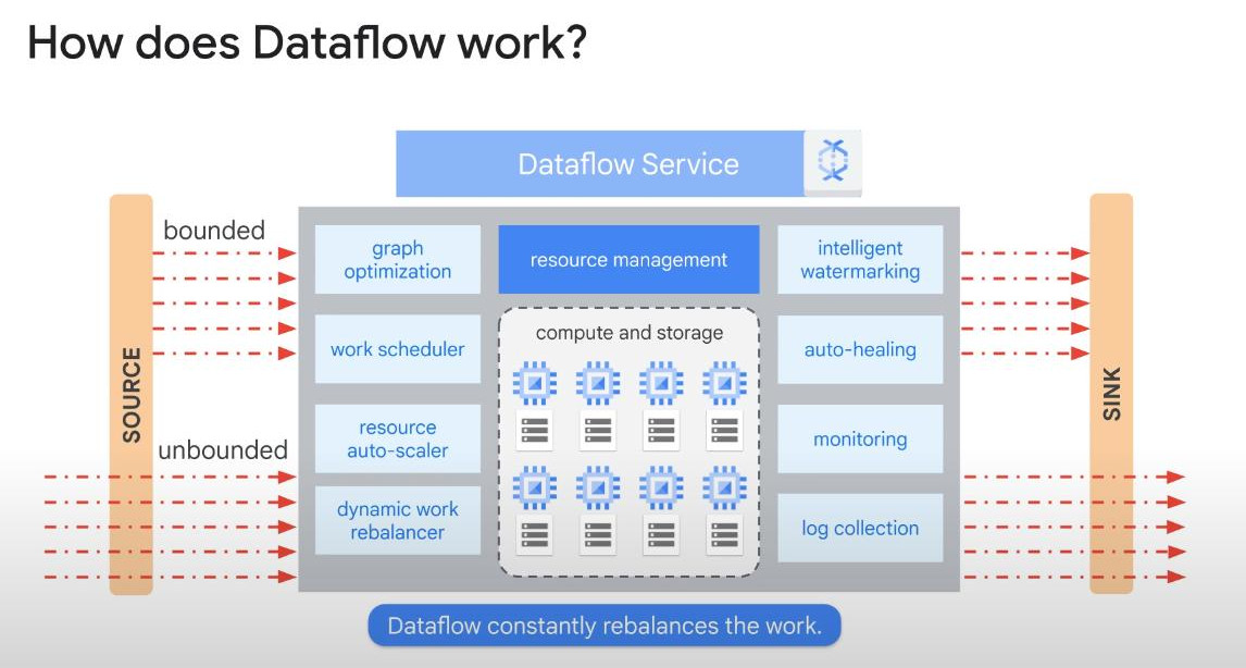
      • How Dataflow works:
        • It is fully-managed and auto-configured,
        • Optimizing the graph continuously,
        • Processed data in parallel,
        • Auto-scaling (more jobs, auto provide more working nodes as necessary)
        • Re-balancing mid-job: one machine after finishing job 1 will be managed to handle other jobs.
        • Able to handle late arriving records with watermarking.
        • Easy to connect with other Cloud services.

      

      • Dataflow Pipeline in Code:

      

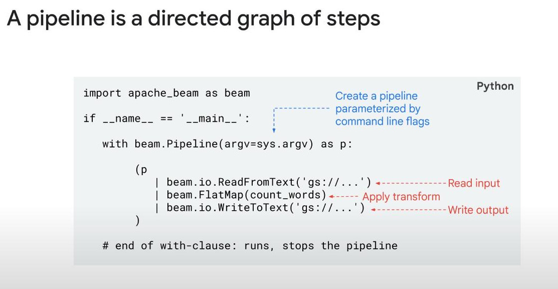
      • Run a dataflow pipeline: (not a prefered way of programming at scale)

      

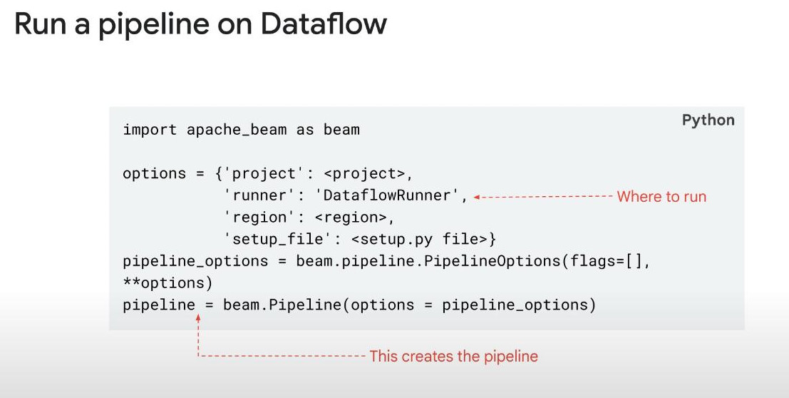
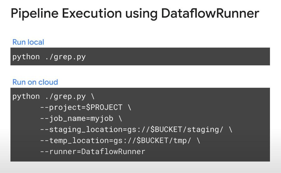
      • Run a dataflow pipeline either locally or on cloud: (specify cloud parameters)

      

      • Design a dataflow pipeline : read data from multi-sources.

      

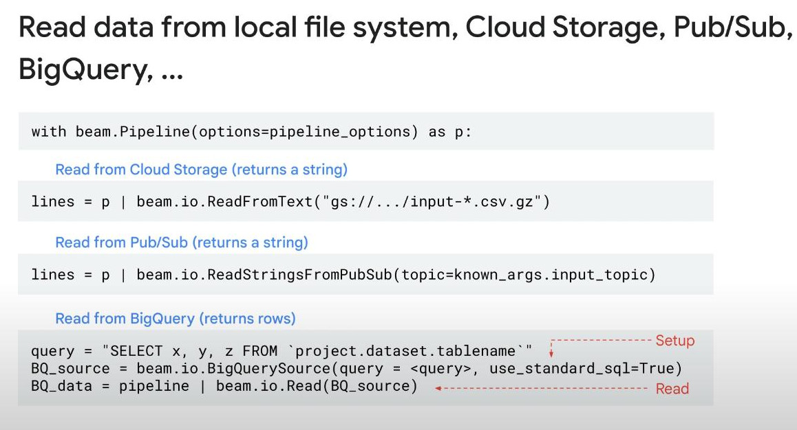
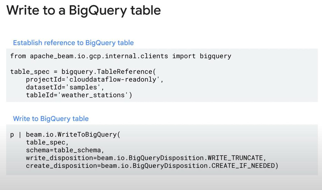
      • Design a dataflow pipeline : Write data to a BQ table:

      

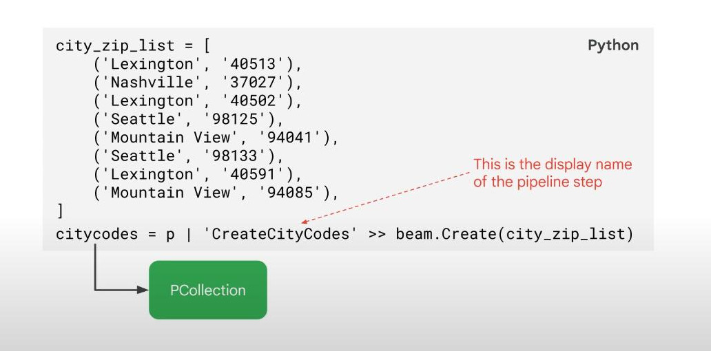
      • Design a dataflow pipeline : hardcode to create PCollection:

      

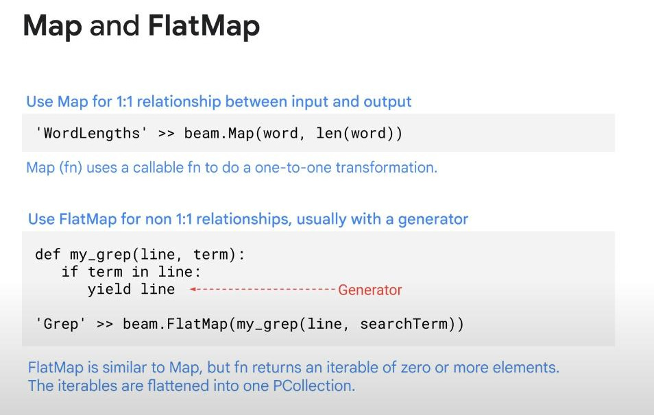
      • Map() vs FlatMap() in PTransform of a Dataflow Pipeline. With Map(), each input element produces exactly one output element. With FlatMap(), each input element can produce zero, one, or many output elements.

      

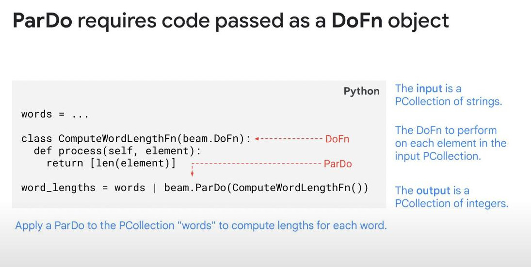
      • ParDo() in PTransform: we can use ParDo() to perform a simple or complex computation with every batch (input). With ParDo(), we need a DoFn object, which is a BEAM class. Specifically, Map() or FlatMap() are just a simple type of ParDo() for transformation. Use ParDo() when you need more complex transformation.

      

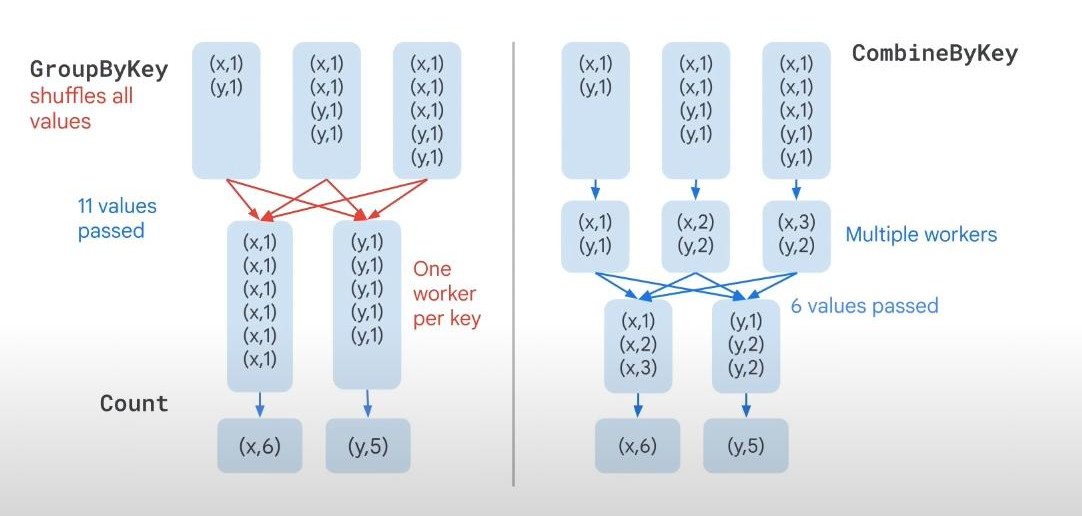
      • Dataflow Aggregation with GroupByKey and Combine (Reduce): after mapping (Map()), we can combine or group data together: (k1,v1), (k1,v2), (k1,v3) -grouping-> (k1, [v1,v2,v3]). This happens on PCollections:

        • GroupByKey(): operates on one PCollection for grouping. It can become in-efficient with data skew. It means one key has too many values compared to other keys, leading only one worker node, other worker nodes are idle (waiting but still costing).
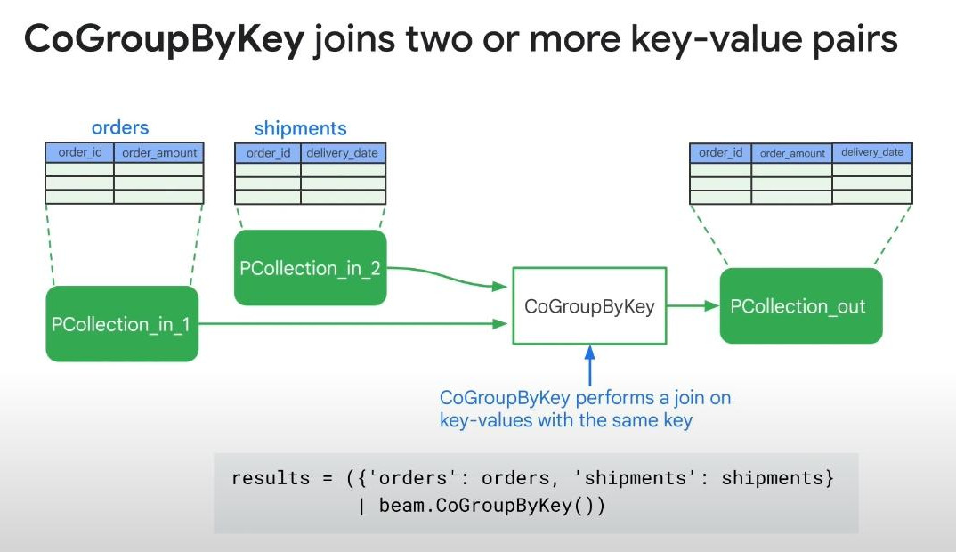
        • CoGroupByKey(): operates on multiple PCollections for grouping. After doing GroupByKey() on each PCollection, now we can combine several PCollections together if they have a same key.

        

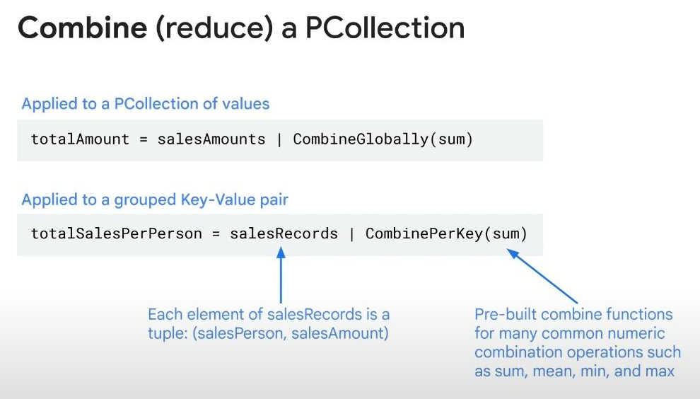
        • Combine phase = Reduce: it can be CombineGlobally(sum), CombinePerKey(sum). Some simple combine methods are pre-built like sum, min, max.

        

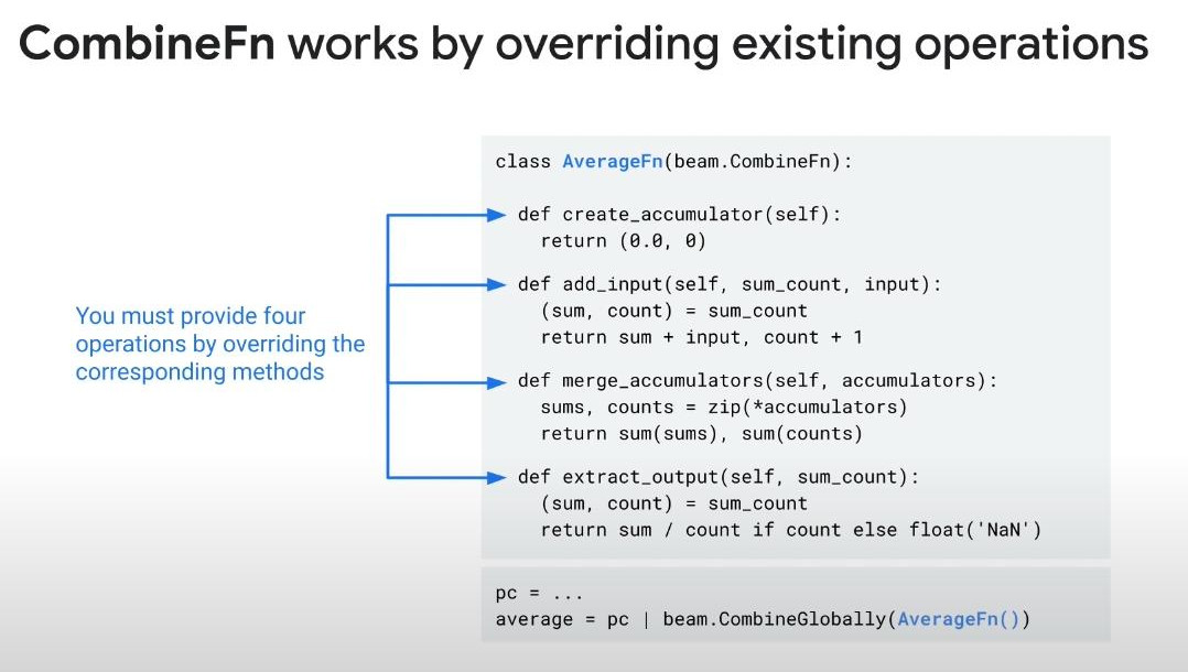
        • More complex require customisation with a subclass of a combine:

        

        • Combine is more efficient than GroupByKey. It is because one worker only can work with one key in GroupByKey, Combine does not have that limit.

        

        • Flatten() : merges identical PCollections storing same datatype into one.
        • Partition() : split one PCollection storing same datatype into several PCollections.

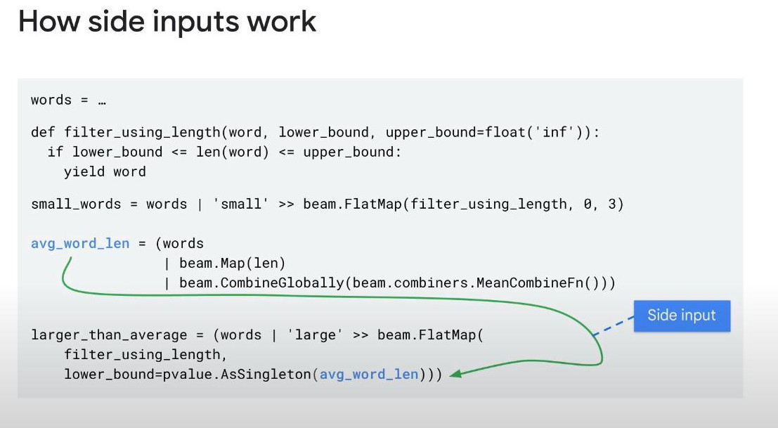
      • Side inputs and windows of data:

        • Side inputs: during creating a PCollection, we can inject additional data during the runtime of ParDo() transform-function. A side inputs occurs each time of processing a new element in the PCollection, so the additional data needs to be determined at RUNTIME, not hard coded.
          • But why we need sideinput? If we want the same result without using the _side_input transform, we have to join the main data with the sideinput data, this JOIN would be very expensive if _side input data is small, but if this JOIN should be re-considered again when the side input data is over 100MB.

        

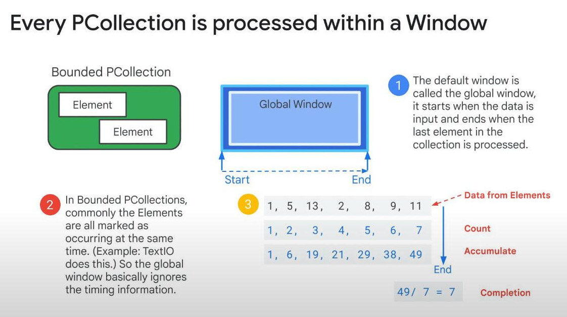
        • What is the Window of data: For bounded PCollection, the default window is called the global window, that is not time-based but it can ends when the last element of the bounded PCollection is processed. We can set it manually.

        

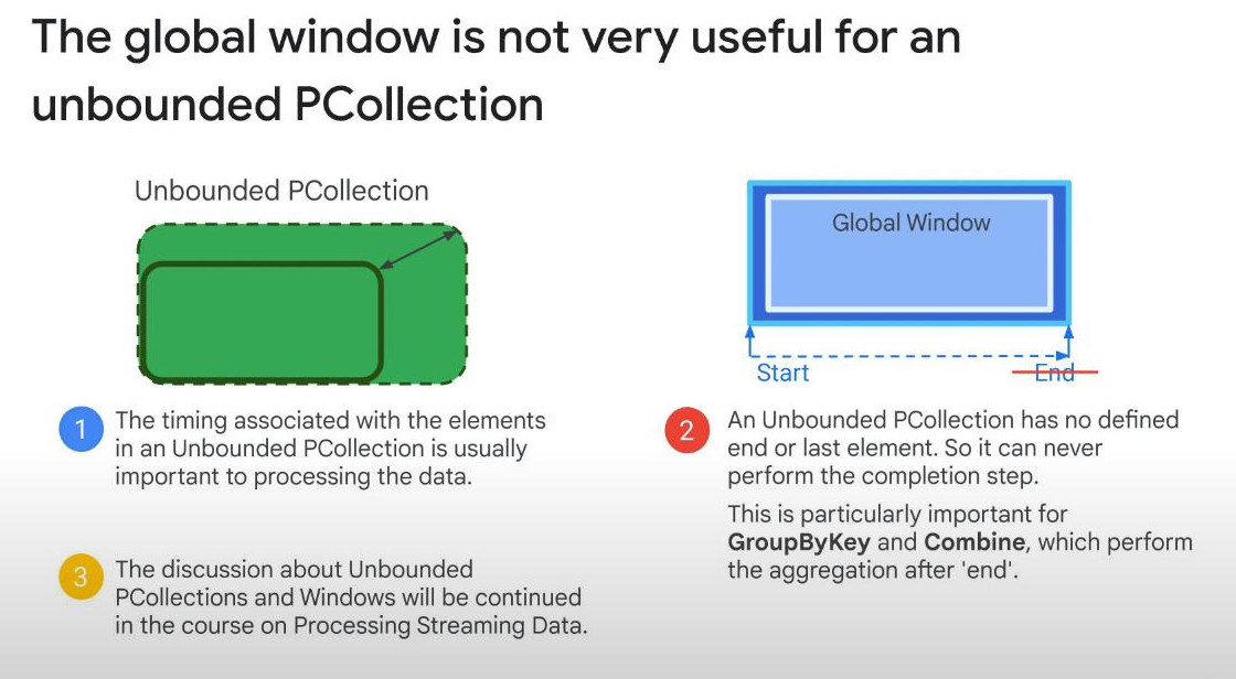
        • Warning: the global window is not effective for streaming data or unbounded PCollections. Unbounded PCollection has no defined END or last element, this also influences GroupByKey and Combine. For streaming data (time-series data), we can use Time-based Windows.

        

        • For Batching: we also can use time-based Windows as well. “60,30” means capture data in 60s but start a new window every 30s.

        

      • Dataflow Templates: enable users who dont have any coding capability to execute a dataflow job. Developer build templates that dataflow will store in Cloud Storage, then normal user can submit them to run jobs. This does not need to re-compile as re-running a job. You can use available Google Templates or create your own templates. Runtime parameters are necessary as run a template such as input and output below.

        •   args, beam_args = parser.parse_known_args()
            with beam.Pipeline(argv=beam_args) as p:
                (p  | 'ReadFromGCS' >> beam.io.ReadFromText(args.input)
                    | 'WriteToGCS' >> beam.io.WriteToText(args.output))
          

        
        - Execute a dataflow template from Cloud Shell with some *runtime parameters*:
        
        - ```sql
            gcloud dataflow jobs run my-job-instance \
            --gcs-location gs://my-bucket/templates/my_template \
            --region us-central1 \
            --parameters input=gs://my-bucket/data.csv,output=gs://my-bucket/output/
        

    • DATAFUSION: designed for batch data and streaming data pipelines.

      • DataFusion helps build visually or graphically data pipelines. It is a no-code tool to build a data pipeline.
      • Integrate with any type of data.
      • Can combine all data from different sources into one like BigQuery, Spanner,…
      • Reduce complexity.

      • Allow create templates.

      • Components of DataFusion:

        • Wrangler UI is a framework for exploring datasets visually and also building data pipelines with no code. (wrangle data: transform and clean raw data)

        

        • Data Pipeline UI is a framework for drawing pipelines onto a canvas.

        • Rules Engine is a tool to build rules
        • Metadata Aggregator is a tool to analyze complex metadata.
        • Microservice is a framework to build a specialized logic to process data.
        • Event Condition Action -ECA is an application to
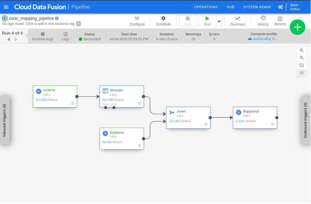
      • Running a pipeline after builsing and deploying:

      

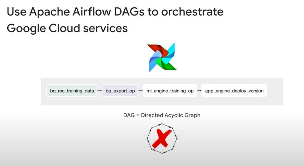
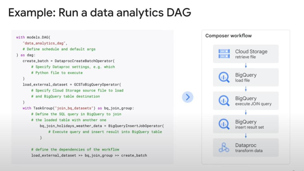
    • CLOUD COMPOSER: if we want to run 3 data fusion pipelines and 2 ML models training in a certain order, we need Cloud Composer like an orchestration engine.

      • Cloud Composer is a serverless environment where a DAG workflow tool runs. That DAG workflow tool is called Apache Airflow, an open-source orchestration engine. Like Datafusion, we will build a DAGraph again, yes, we can build almost anything with it.

      

      • Keeping mind that, we can have multiple Cloud Composer environments, each contains one separate instance of Apache Airflow, which could have many DAGs.

      • When we create a Cloud Composer instance, a Cloud Storage bucket will be automatically created to store DAG file written in Python or Airflow workflows are written in Python.

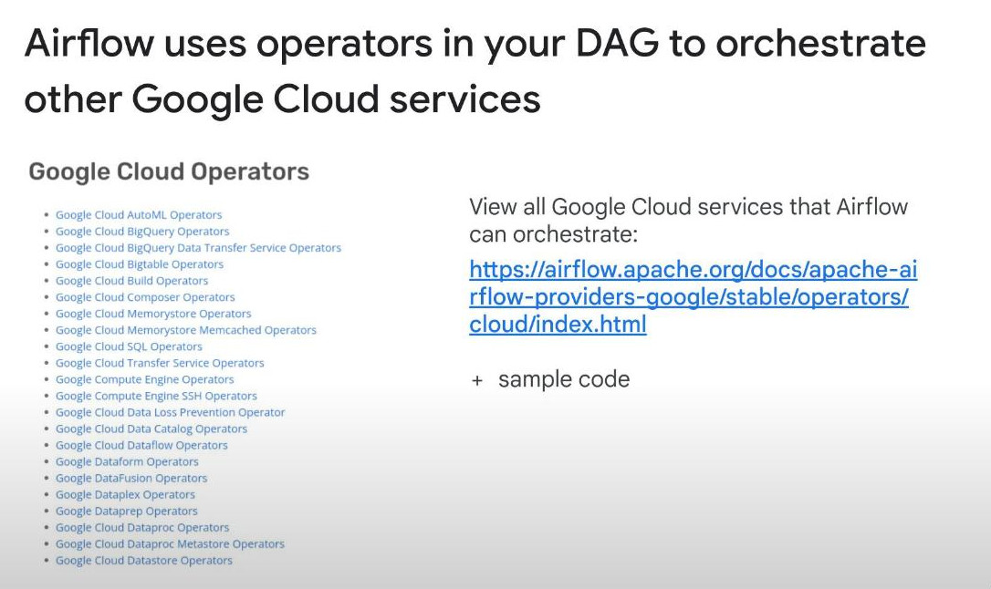
      • Operators in Cloud Composer are pre-built tasks that perform specific actions. In other words, operators are fundamental building blocks that define tasks in DAGs (Directed Acyclic Graphs).

      

      

      • Apache Airflow is an open source and continuously add more operators, be sure to check out new operators. Apache_Airflow_GitHub_Repo and Official_AirFlow_Website.

      • Workflow Scheduling : there are 2 types: periodic & event-triggered.

      

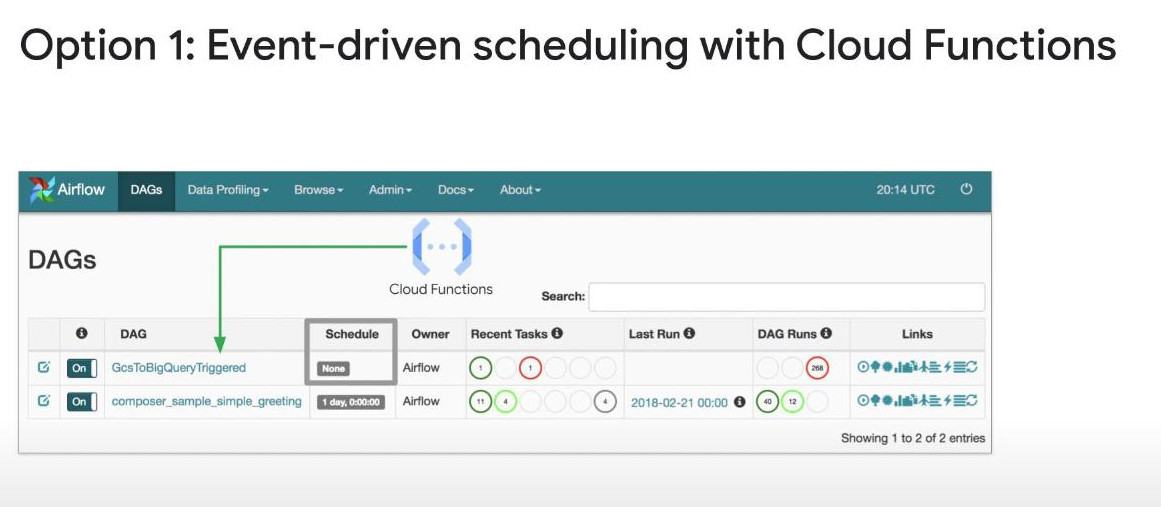
      • We can check whether DAGs worked like schedulings or not, by checking the log files.

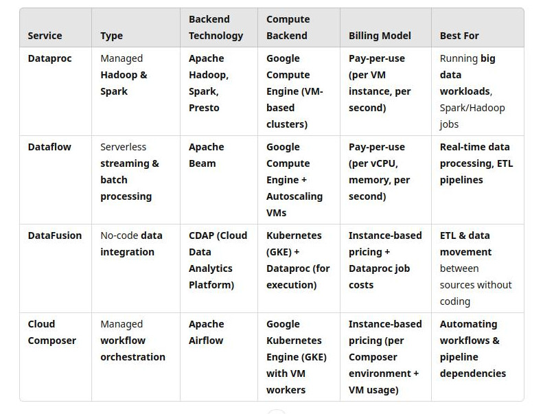
    Finally, we can see the key difference between dataproc, dataflow, datafusion and composer:

    

    • STREAMING DATA & ANALYTICS SYSTEMS:

      • Why streaming : help make decision at real-time.
      • Streaming is data processing for unbounded data set.

      • Challenges associated with streaming applications: we have 4Vs (variety, volumne, velocity and veracity (tính chân thật)).

        • Variety: data can come in various formats or sources.
        • Volumne: from gigabytes to petabytes.
        • Velocity: streaming should be a near-real time process.

      • 3 main services in streaming Data process: Pub/Sub, DataFlow, BigQuery.

      • Pub/Sub: Pub/sub does streaming differently than almost anything you have used in the past.

        • a fully managed data distribution and delivery system.

        • Pub/Sub is not a software, it is a service. So, Pub/Sub client libraries are available in many programming languages (Java, C#, Pyhon, Ruby,…).

        • 3 qualities of the Pub/Sub service:

          • Availability:
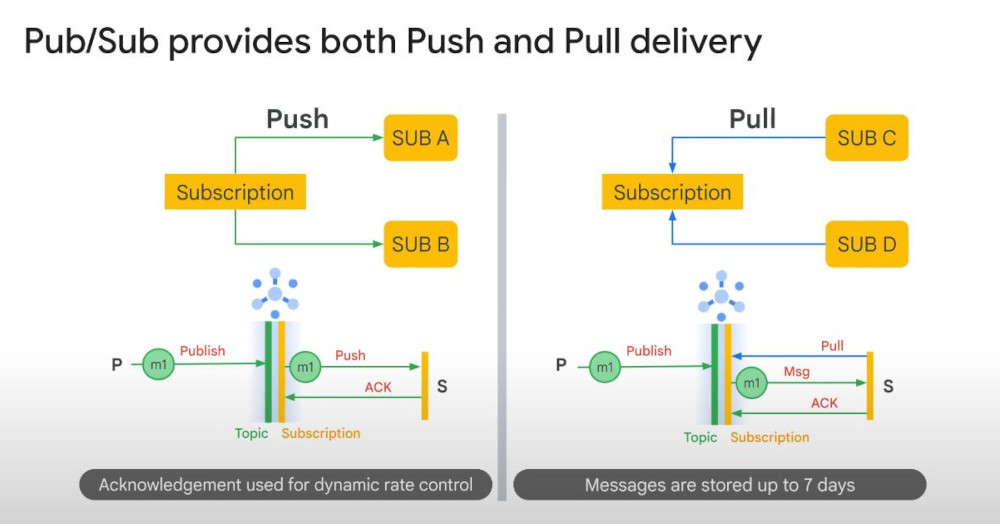
          • Durability: by default it saves our messages for 7 days.
          • Scalability: Google Cloud processes about 100 million messages per seconds. On average, Google is indexing the web 03 times/day. Thus, Google is sending the entire web over Pub/Sub 03 times/day.

        • We can control the qualities of Pub/Sub by the number of publishers, number of subscribers, the size and number of messages.

        • Pub/Sub is a story of 2 data structures, the Topic and the Subscription:

          • A decoupling system: an architecture where services/modules are loosely connected instead of tightly integrated.

          • The Pub/Sub client that created the Topic is called publisher.

          • The Pub/Sub client that creates the Subscription is called subscriber. To create a message to the Topic, we need a Subscription to that Topic. One Topic can have multiple subscriptions or Subscriber apps.

          

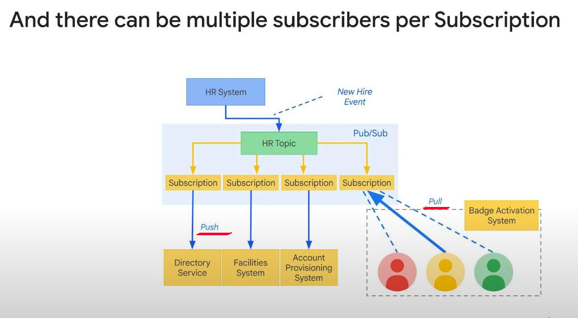
          • Push process: Pub/Sub sends messages to the subscriber’s endpoint (e.g., HTTP webhook).
          • Pull process: The subscriber requests messages from Pub/Sub when ready.

        • Google Pub/Sub takes the highest priority in managing and updating latest information directly in any systems.

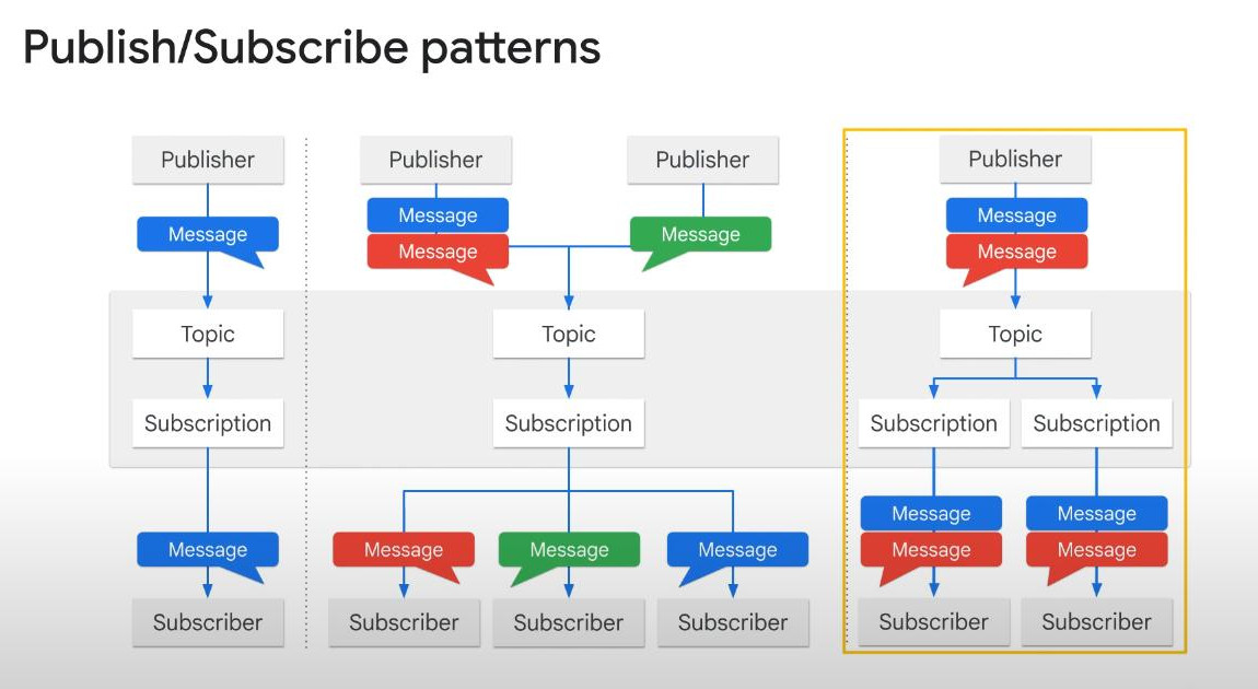
        • Generally, there are 3 main Pub/Sub patterns:

        

        • Acknowledgement (Ack) : in Google Cloud Pub/Sub, ack ensures that messages are successfully received and processed by the subscriber. If a message is not acknowledged, Pub/Sub retries sending it until the retention period expires (default 7 days).

        

        • Ack deadline : is the maximum time a subscriber has a acknowledge a received message and send this ack to Pub/Sub, then the message is removed from Pub/Sub. Otherwise, Pub/Sub re-deliver the message.

        • Message Replay : we can ask Pub/Sub to published again all messages within 7 days, even acknowledged ones. For this, we need to enable message retention in Pub/Sub to make sure acknowledged messages are not removed. Replay is useful when a subscriber failed to process messages correctly.

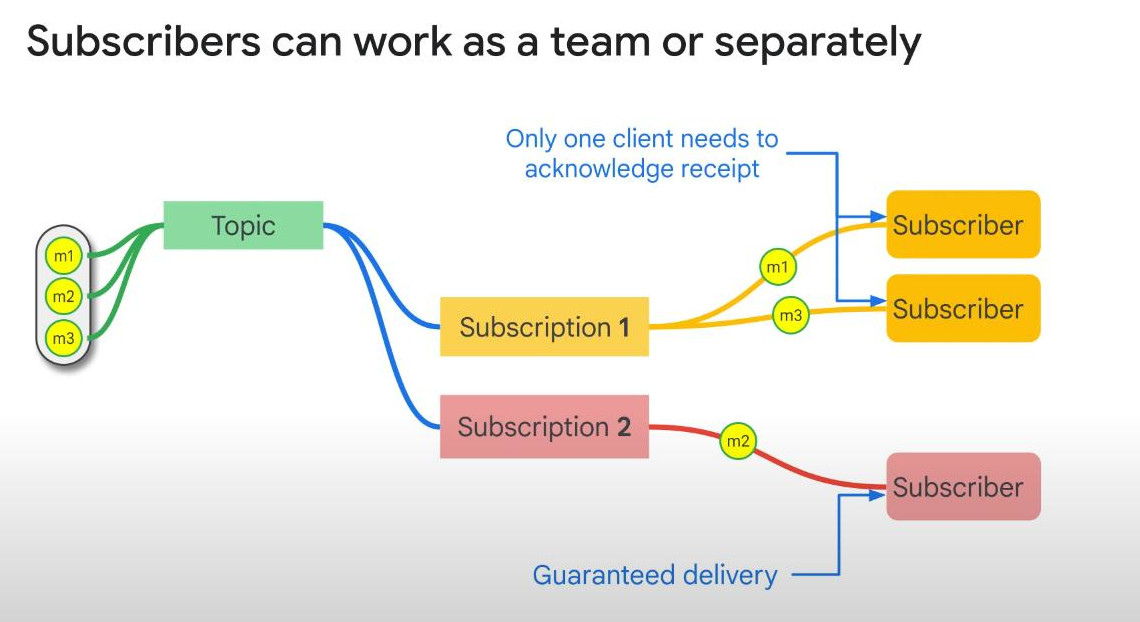
        • Subscribers can work as a team or separately. In a team, only one subscriber has to acknowledge the message receipt.

        

        • Message order: By default, Pub/Sub does NOT guarantee message order because messages can be processed in parallel across multiple subscribers. However, ordered message delivery can be achieved using ordering key. (Note: this increases the latency).

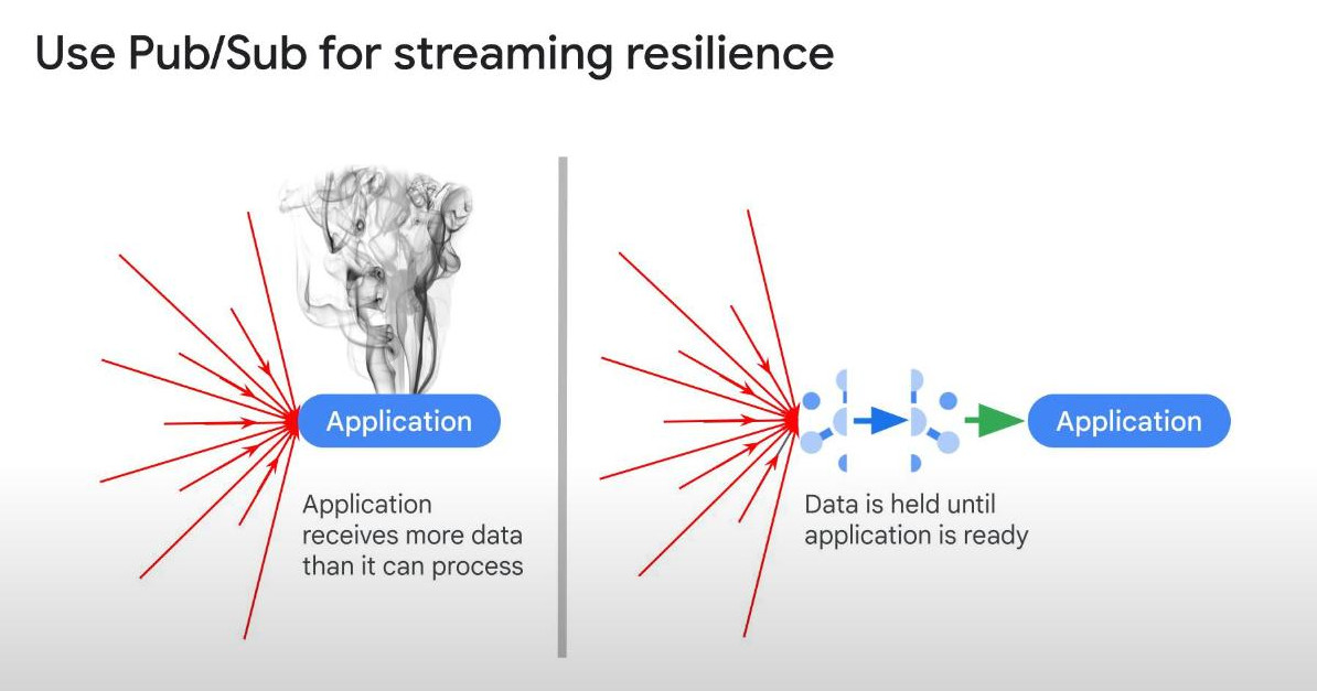
        • The important role of Pub/Sub for streaming resilience: for examples, data can explode on black Friday or subscriber could fail for 1 day.

        

        • Dead-letter Queue DLQ : a Pub/Sub feature that stores messages that fails to be processed multiple times. Instead of being loss, they are redirected to a separate Pub/sub topic “Dead-Letter” for future debugging some manual action. This feaure helps prevent infinite retries. (recommended).

        • Exponential Backoff : is a retry strategy where the wait time between retries increases exponentially (lũy kế) after each failure. This helps reduce system overload, prevent thundering herd issues, and improve resilience.

    • DataFlow in STREAMING : what is the challenges:

      • Challanges as streaming:

        1. Scalability : data only grows larger.
        2. Fault tolerance :
        3. Model : streaming and repeated batch.
        4. Timing : how to deal with latency?

      • Dataflow helps divide the stream into a series of finite windows, so we can use the original timestamp of pub/sub messages to add the messages into different time windows, even if they arrive late or out of order, so we can still group the messages correctly.

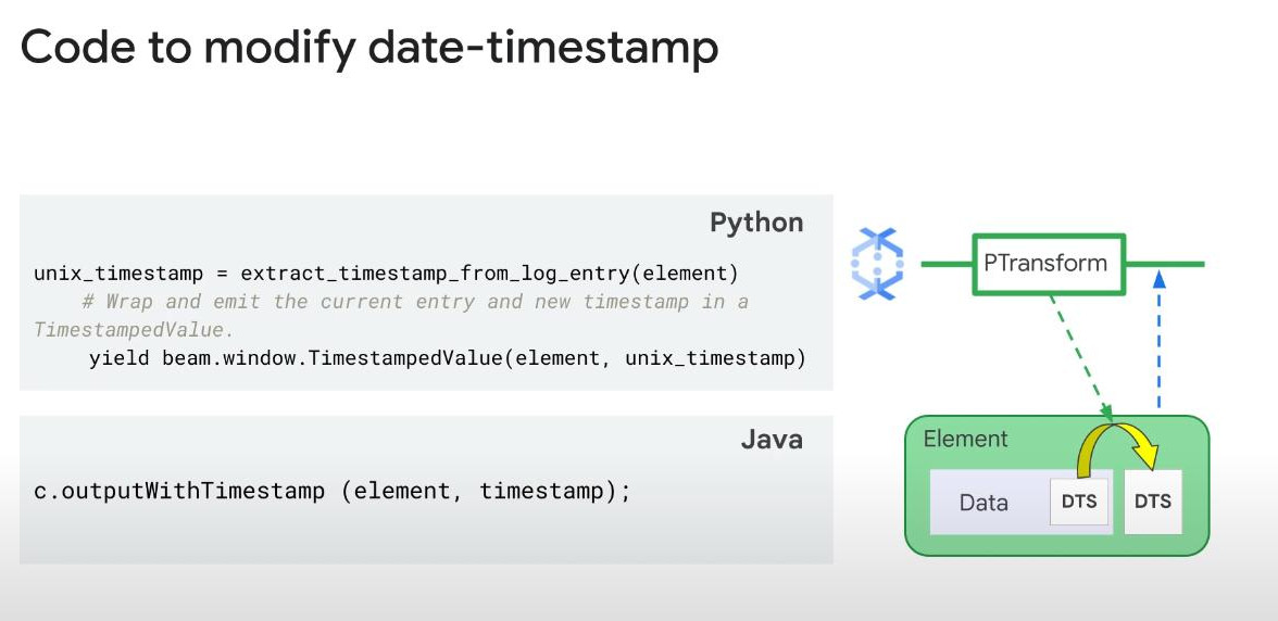
      • Modify the date-timestamp (DTS) with a PTransform if needed because every message always have a timestamp in its metadata which is provided by the pub/sub sensor as pushing. This timestamp will be different from the time when Dataflow receive the message. PTransform can use this DTS to modify the timestamp at Dataflow.

      

      • Duplicate messages with custome IDs: if Pub/sub IO is configured to user custom Ids for messages, Dataflow will maintain a list of all messages during 10 minutes, if a new message’s ID is in the list, the message is assumed to be duplicated and be discarded.

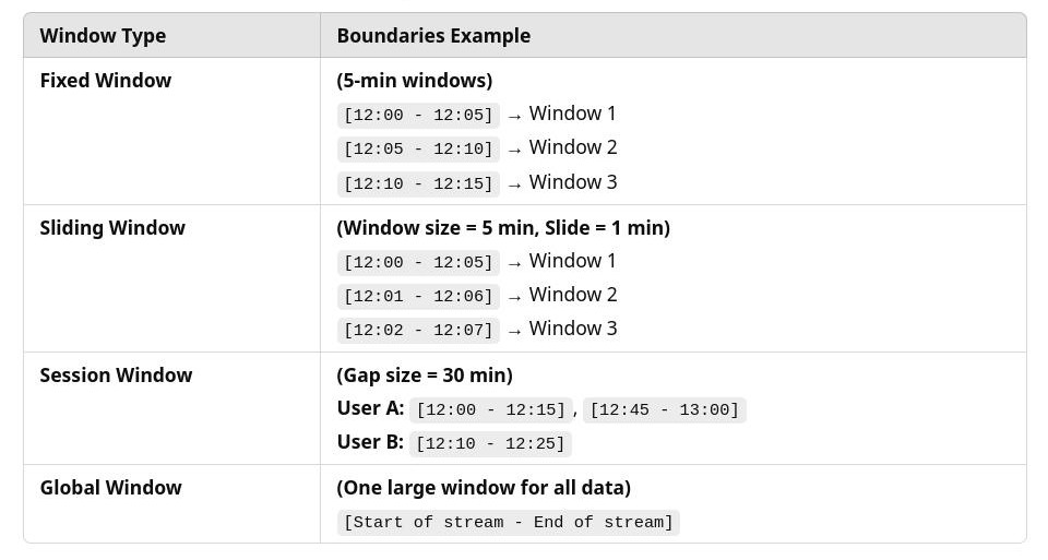
      • Dataflow windowing : Dataflow provides 3 kinds of windows fit most circumstances:

        1. Fixed window (Tumpling): contains no overlapping intervals.
        2. Sliding window (Hopping): sliding time windows can overlap if the slide time is smaller than the window size because events will appear in multiple windows.
        3. Sessions window: defined by user activity, dynamically sized. If the gap is set 10 minutes, only when there’s no user activity over 10 min, the session will closes autmatically and a new session starts. If user activity keeps happening or never stop longer than 10 minutes (gap), current session window can extends longer and longer.

      • In an ideal world without network latency, we have some examples like the following table.

      

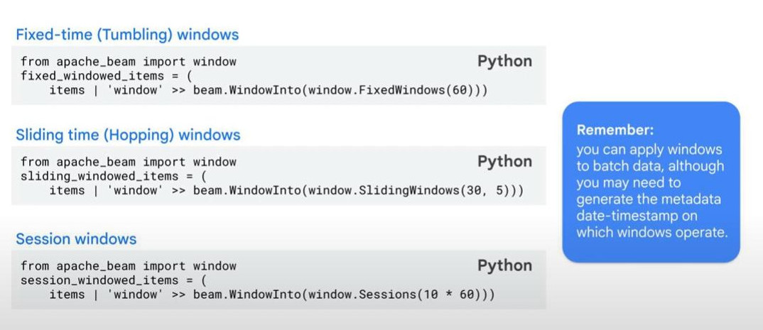
      • Code to set Dataflow windows in Python:

      

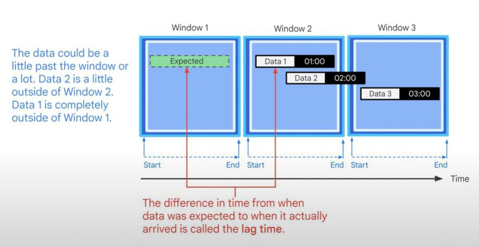
      • Lag time: With latency in the real world, under delay influence, we can have some some small or large lag time:

      

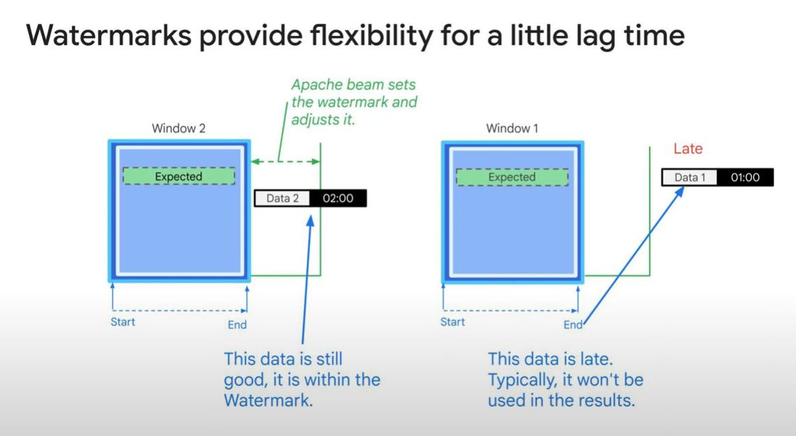
      • Watermark: watermark is a tool to deal with lag time:
        • A watermark represents the point in event time where Dataflow assumes all earlier events have been processed.
        • Events arriving after the watermark are considered late but may still be processed (depending on allowed lateness).

      

      • By default, data later then watermark (a threshold) will be discarded or handled separately, but we can allow late data past the watermark by setting “allowed_lateness=Duration(seconds=2 _ 24 _ 3600)” that means Dataflow still wait for data of a window for 2 days since the window closes.

      • Custom Triggers : A trigger defines when dataflow should process data to give some output results from a window. Because streaming data arrives almost forever, dataflow cannot wait forever.

      

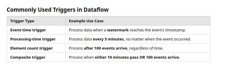
      • Trigger examples:

      

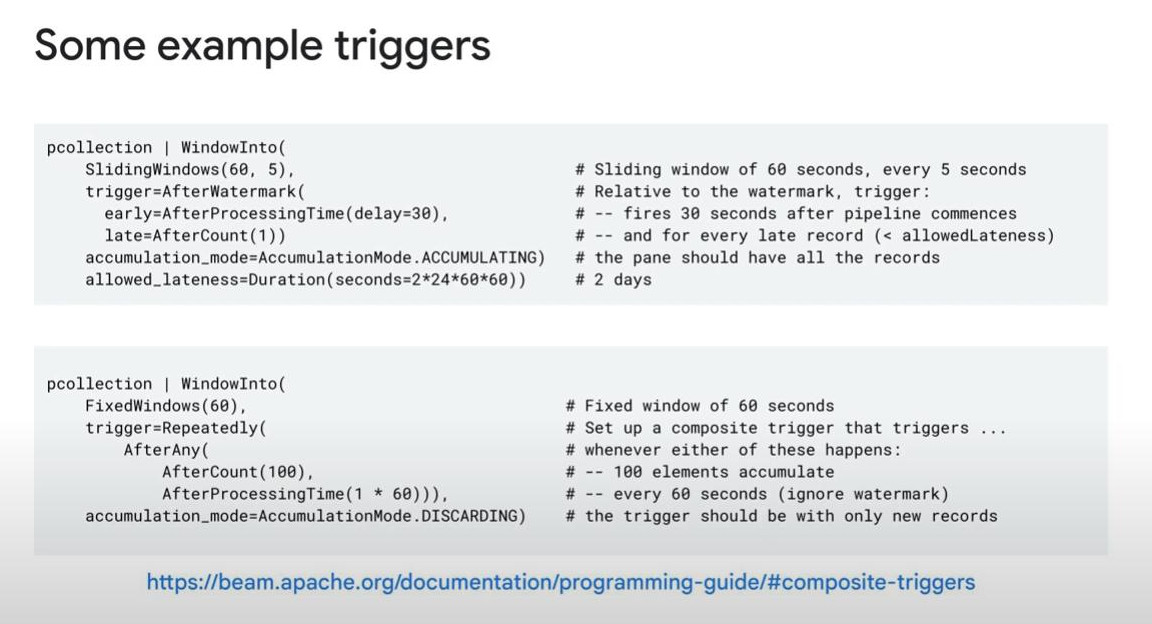
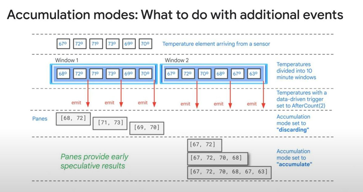
      • Accumulation Mode: just select or not

      

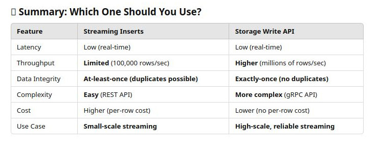
    • Streaming Inserts : they are separate methods of Bigquery used to add streaming data into a BQ table. There is a cost for streaming inserts:

      • Streaming Buffer : data is held briefly “streaming buffer” until it can be inserted into a BQ table.
      • Streaming quotas : Because streaming is unbounded, we need to consider “streaming quotas”. There is both daily limit and a concurrent rate limit. Daily limit is the total amount of messages that can be processed per day. BigQuery Streaming has a daily insert limit of 1 TB/project (1000 GB/project). If we exceed this, we have to wait until the next day. Concurrent rate limit is 100,000 rows/second, if there are over 100,000 messages at the same time, some delay or rejection will occur.

    • Storage Write API is an altenative for “Streaming Inserts” as adding streaming data into a table. It has different quotas, not daily limit or concurrent rate limit anymore. It has 2 throughput quotas, 3GB/sec for multi-region and 0.3GB/sec for single-region. It can be millions rows/sec.

    • How to choose between “Streaming Inserts” or “Storage Write API”:

    

    • When to choose between “ingested stream of data” or “batch data loading”: The answer depends on how much the immediate availability of data is required. Batch data loading is not charged in most cases.

    • Code for Streaming Inserts:

        bq_client = bigquery.Client(project="PROJECT_ID")
        dataset = bg_client.dataset('DATASET_ID')
        table  = bq_client.get_table(dataset.table('TABLE_ID'))
        errors = bq_client.insert_rows(table, rows_to_insert_data)
    

    • Looker Studio:

      • We can have any or all kinds of datasources in a single LookerStudio Report.
      • Reports can be shared and datasources can also be seen, so be careful that anyone, who can see the report, can potentially see all the data of the datasources associated.
      • free and drad-and-drop interface.
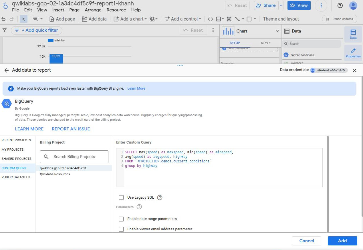
      • From Looker, we can add new data by selecting “Add data” btn => BigQuery => “Custom Query” => ProjectId, issuing a SQL query to BigQuery table into a temp table as a new data source, being seen in tab “Data source” at the “Chart Setup”. Then, we can make a report with this Data source.

      

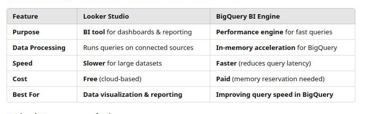
    • BI engine (BigQuery Engine) : It is in-memory layer for BigQuery, meaning in-memory processing avoiding re-scanning data repeatedly. But it is not free and only work with BQ. We have to enable it and allocate memory for it. BI Engine is best when dashboards or Looker need fast, repeated access to the same data, not for data that changes regularly.

    • Compare Looker and BI engine:

    

    • Sending Email By a continuous Query: link

    • bq-continuous-query-sa : a BigQuery service account which is related to BigQuery Continuous Queries, allowing running queries on streaming data, meaning running a query continuously in the background, ensuring real-time analysis or timely actions.

    • Bigtable

      • it is used in cases we need to handle very low latency or very high throughput requirements when BigQuery is not enough.

      • Bigtable is a NoSQL database, meaning Bigtable is not good for data processing that needs SQL queries such as joins, aggregations.

      • ROW KEY : Bigtable has only one index called the Row Key. When new data arrives, it is stored in a MemTable in memory, when it is full, it is then written into disk in a format of dictionary-order by the Row Key.

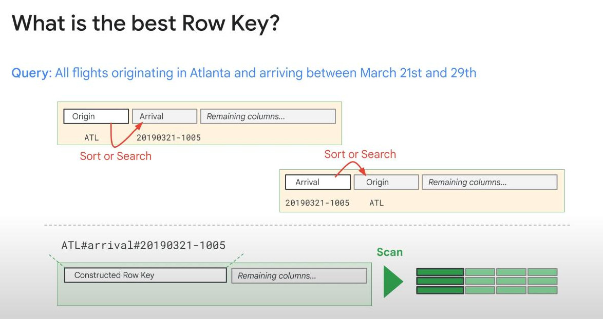
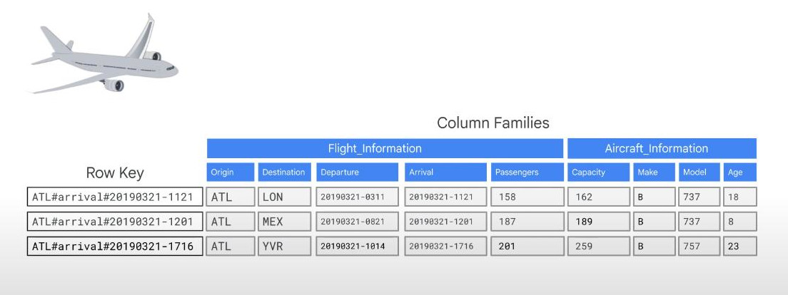
      • CONSTRUCTED ROW KEY : To get the best performance with the design of the Bigtable, we need to get our data in order first, if possible, we need to select and contruct a ROW KEY that minimizes sorting and searching and turns our most common queries into scans, in most cases ROW KEY is a constructed or composite type that is composed of 2 columns, usu one of them is TIMESTAMP. Not all data and not all queries are good use cases for the efficiency that Bigtable offers. But when it is a good match, Bigtable will be very fast like a magic. Like image below, with a constructed ROW KEY (origin-arrivalDate), we only need scanning without any sorting and searching because we did sorting as writing already.

      

      • Column Families : we can devide columns into different groups called “families”, helping access more faster because we only fetch data from one family instead of all families (all columns). Bigtable can handle up to 100 column-families without losing performance.

      

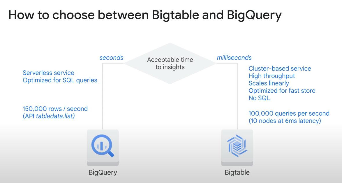
      • BigQuery is serverless, Bigtable is cluster-based. How to choose, Bigtable or BigQuery.

      

      • Bigtable stores data in file system called “Colossus” that contains tablets, a data structure to identify and manage data (a number of contiguous rows within a table). Tablets’metadata is stored in VM nodes of Bigtable cluster, leading 3-levels of operation: manipulate the data, manipulate the tablets, and manipulate the metadata.

      • SELF-IMPROVES with POINTERS : Bigtable periodically rewrites our table to remove deleted entries and to reorganize data, ensuring reads and writes remain efficient. It tries to distribute reads and writes equally across all Bigtable nodes in the cluster. In nature, it just moving the POINTERS across nodes (pointers are not data but references or cache). It doesn’t move all rows, just its pointers. Actual data is located in Tablets. To be more clear, if only certain rows are accessed more frequently than others, we can get balancing by distributing their tablets across the nodes.

      • Re-balance STRATEGY is to distribute reads: notice that even distribution of reads takes priority over evenly distributing storage.

      • How to optimize a Bigtable performance: there are serveral factors that can result in slower performance:

        • The table schema design is not correct. It’s essential to design a schema that allows reads and writes to be evenly distributed across the Bigtable cluster nodes. Otherwise, individual nodes can get overloaded, slowing performance.
        • The Bigtable cluster doesn’t have enough nodes. Typically, performance increases linearly with the number of nodes in a cluster. Use Monitoring tools to check whether a cluster is overloaded.

        • Bigtable can be used with HDD disks and SSD disks. HDD disks can result in slower response times and significantly lower number of reads requests/sec, 500 QPS/sec for HDD disks, 10000 QPS for SSD disks. In 2024, a 10-node SSD cluster with 1KB rows (each row is 1KB) and “write-only workload” can process 10,000 rows/sec at a 6-milisecond delay.

        • Network issues can cause reads and writes to take longer than usual. Network issues often happens if clients is not at the same zone as Bigtable cluster.

        • Different workloads could cause performance to vary. We should perform some tests to obtain the most accurate benchmarks. For example, throughput can be controlled by node count. With 100 nodes, we can handle 1 million QPS (Queries per seconds). A higher throughput means more items are processed at a given amount of time.

        • In general, smaller rows offer higher throughput, and therefore are better for streaming performance. Bigtable takes time to process cells within a row.

        • Selecting the right ROW KEY is critical. Rows are sorted lexico-graphically (in dictionary-order).

        • Avoid “hot spots” during “Writes Streaming”: ‘hot spot’ issue can be there are too many write requests on the same rows or same tablet. It can also be one node handle most writes. For ex, “timestamps” or “IDs” are naturally sequential, leading easily new writes will target the same node or same tablet if our ROW KEY is configured with only timestamps. We should use composite ROW KEY like “typeA#timestamps”, “typeB#timestamps”, so new writes can be distributed more evenly across nodes.

        • Replication for Bigtable is to increase the availability and durability of our data by copying it across multiple regions or multiple zones within a same region. Replication will allows us to isolate workloads by rounting different types of requests to different replicas. Failover is used to automatically redirect requests to healthy replicas in case one replica was broken. Bigtable supports automatic failover for high availability. But “isolating workloads”, “increasing number of nodes”, “decreasing row size and cell size” are not automatic. We need experimentation to find the best solution.

        • The ability of create multiple clusters in an instance is valuable for performance, as one can be for reads and one replica is exclusively for writes.

        • 300 GB is the min data volume to run a test on Bigtable.

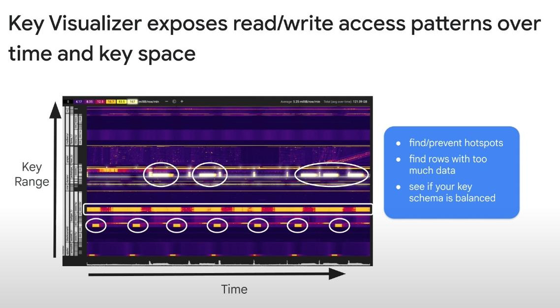
      • Key Visualizer is a heat map (Ox:time, Oy:row keys, higher values appear in white color) that automatically generates hourly and daily scan for every table that meets at least one of the following criteria:

        • 1. During the previous 24 hours, the table contained at least 30 GB of data at some point of time.
        • 1. During the previous 24 hours, the average of all reads or writes was minimum 10,000 rows/sec.

        

    • Bigquery Geo Viz : a lightweight cloud application that allows for quick testing of geospatial data.

      • ST_GeogPoint(longitude,latitude) is a SQL code to convert 2 FLOAT-typed longitude & latitude to a GIS-typed geospatial point (or exact coordinates - toạ độ) on GIS map (Geographic Information System) of Google.

      • ST_GeogFromGeoJSON(longitudeJSON, latitudeJSON): similar to ST_GeogPoint() with JSON format.

      • ST_Distance(p1, p2): distance between 2 points. (p1,p2 is GIS-typed point from ST_GeogPoint()).

      • ST_MakeLine(point1, point2) will overlay a line between 2 geospatial points on a map.

      • ST_UNION_AGG(lines): aggregate all the lines from ST_MakeLine()

      • ST_MakePolygon(ST_MakeLine([point1, point2, point3])) will also overlay a triangle with 3 geospatial points on a map, helping highlight relationships in the data.

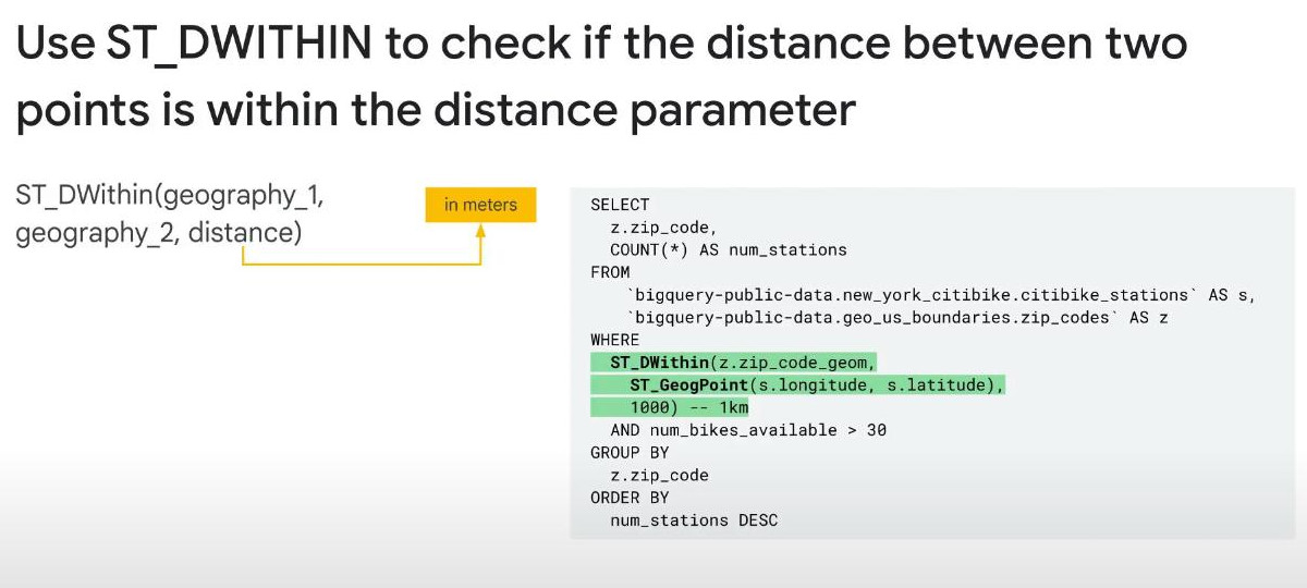
      • WHERE ST_DWithin(point1, point2, 1.5e5) –150km is used to filter out bike stations (point2) within 150km linear distance from point1(a city center or the post office).

      

      • ST_Intersets(polyA, polyB): true if two polies overlap.
      • ST_Contains(polyA, point1): true if a point is inside a polygon.
      • ST_ConveredBy(polyA, polyC): true if polyA is completely inside polyC.

    • BIGQUERY SQL OR PRICING OPTIMIZATIONS: FAST but SMART (smart = not expensive)

      • Best practices we should consider:

        • Use Dataflow to do the processing and data transformations.
        • Create multiple tables for easy analysis.
        • Use Bigquery for streaming analysis and dashboards.
        • Store data in Bigquery for low cost and long term storage.
        • create Views for common queries.

      • Good Data analyts will explore how the datasets are structured even before writing a single line of code.

      • Revisit the schema, make questions: what were the goals then? Are those the same goals at present?. Analogy, for dirty dishes, if you clean them as you use them, the kitchen remains clean. If you save them, you end up with a sink full of dirty dishes and a full of work.

      • 5 key areas of BQ performance optimization: less work == faster query.

        • For Input/Output: How many bytes were read from disks?
        • Shuffling: how many bytes were passed to the next query stage? (one query can have several stages, filtering or sorting or aggregating,…)
        • Grouping: how many bytes were passed through each group.
        • Materialization: how many bytes were written permanently out onto disk?
        • Functions and UDFs (user-defined func): How much CPU (slots) are the functions using?
        • Slogan: don’t scale up your problems, solve them earlier while they are small.

      • Query Structure Best practices:

        • Avoid “select *” or don’t select more columns than you need.
        • Considering “APPROX_COUNT_DISTINCT()” instead of COUNT(DISTINCT…) for a very large dataset.
        • Make liberal use of “WHERE clause” to filter in queries as soon as you can.
        • Don’t use “ORDER BY” in WITH clause or subqueries, only apply “ORDER BY” at the final or outermost stage of a query.
        • For JOIN, put the larger table on the left
        • Note: if we forget those best practices, BQ will likely do it for us
        • can use wildcards in table suffixes to query multiple tables, but keep specific as much as possible.

        •   SELECT *
            FROM `my_project.my_dataset.logs_*`  --wildcards
            WHERE _TABLE_SUFFIX BETWEEN '20240310' AND '20240312';  --specific
          

        • For “GROUP BY”, be careful to avoid data skew as GROUP_BY that possibly results in 30 minutes processing a query in case of different zones. Because some “values” occur many and many times compared to others. Solution: use approximate funtions first, or GROUP BY 2 values to create a balance, or use BI engine (with in-memory processing).

        • Lastly, use partitioned tables if possible.

        • Break a complex query into multiple-staged query with “intermediate table, view or materialized view, even denormalization” to avoid join. Each stage will materialize an intermidiate tables that stores result for next stages. Analogy: flying directly from the USA to Japan versus taking shorter connecting flights. A direct flight must carry all the fuel at once, while connecting flights only need fuel for each shorter journey. In a real context, we must calculate both storage and processing costs. However, storing and processing big data often costs more.

        • Avoid self-joins of large tables, instead we can use aggregation or window functions or trimming data as small as possible before joining.

        

        

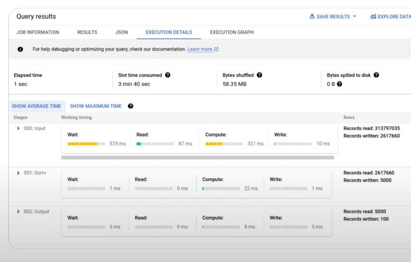
        • Way to check how many bytes or records being processed by clicking on EXECUTION DETAILS tab at BQ UI. It shows the work required to process a job at each stage.

        

        • Another way to analyze a query performance is CLOUD MONITORING: we can check SLOTS UTILIZATION,…

        

        • Use BI engine if you have a dashboard that keeps the exactly same data all the times.

        • PRE-COMPUTATION : sometimes, it can be helpful to precompute functions on smaller tables, and then join with the precomputed values rather than repeat an expensive calculation on a larger tables each time. We need run tests to check.

        • 1.5GB is max for sorting in 2025: First, we need to know sorting is an expensive operantion because Bigquery typically will perform sorting on a single worker, even “LIMIT 10” will not help avoid this because it occurs after sorting is completed. For ex, ROW_NUMBER() OVER(ORDER BY end_date) AS rental_number will do the sorting the entire dataset first required by “ORDER BY enddate”. Therefore, 1.5GB of data is the threshold over which a worker will gets overloaded or overwhelmed while sorting. Solutions are partitioning, clustering by end_date, or approximate ranking with _NTILE(1000) OVER (PARTITION BY MOD(rental_id, 1000) ORDER BY end_date) AS rental_approx_rank to dividing into 1000 groups then sorting and numbering them from 1->1000. In real case, EXTRACT(DATE FROM end_date) is used to reduce sorting complexity because we only check DATE not TIME anymore.

        • APPROX FUNCTIONS’ACCURACY : approximate functions is much more efficient than the exact algorithm only on large datasets and is recommended in use-cases where errors of approximately 1% are tolerable.

    • Compare ETL options

    

11. Automation Tech: (How to automate a Dataflow template)

    • Both ETL or ELT can be automated on a recurring (parameterization) basis.

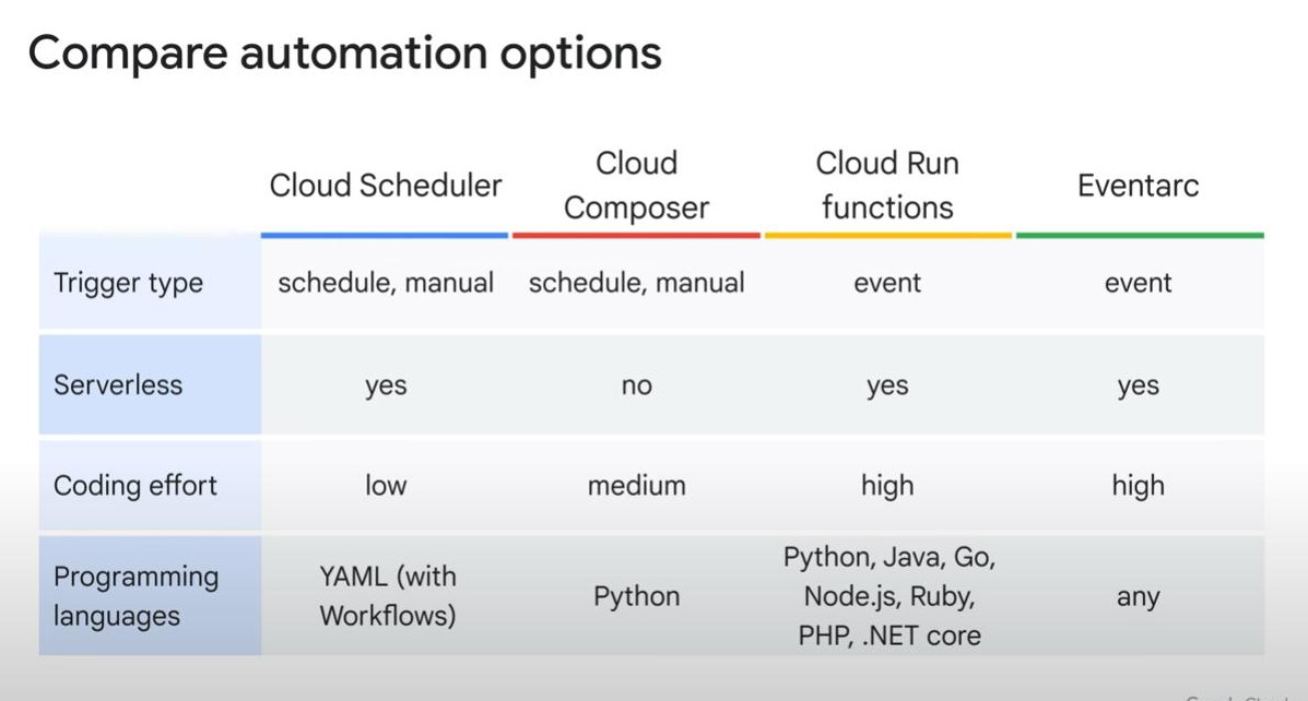
    • 3 common types of Automation: One-off (schedule), Workflow orchestration, Event-based execution.

    • Cloud Scheduler is a automation tool. Trigger can be Http calls, Pub/Sub, Workflows Http.

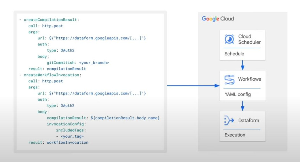
    • Example: Trigger a Dataform SQL workflow. (Yaml file)

    

    • Cloud Composer is to compose data pipelines on different systems, using Apache Airflow.

    

    • Cloud Run allows to execute code based on GC event.

    

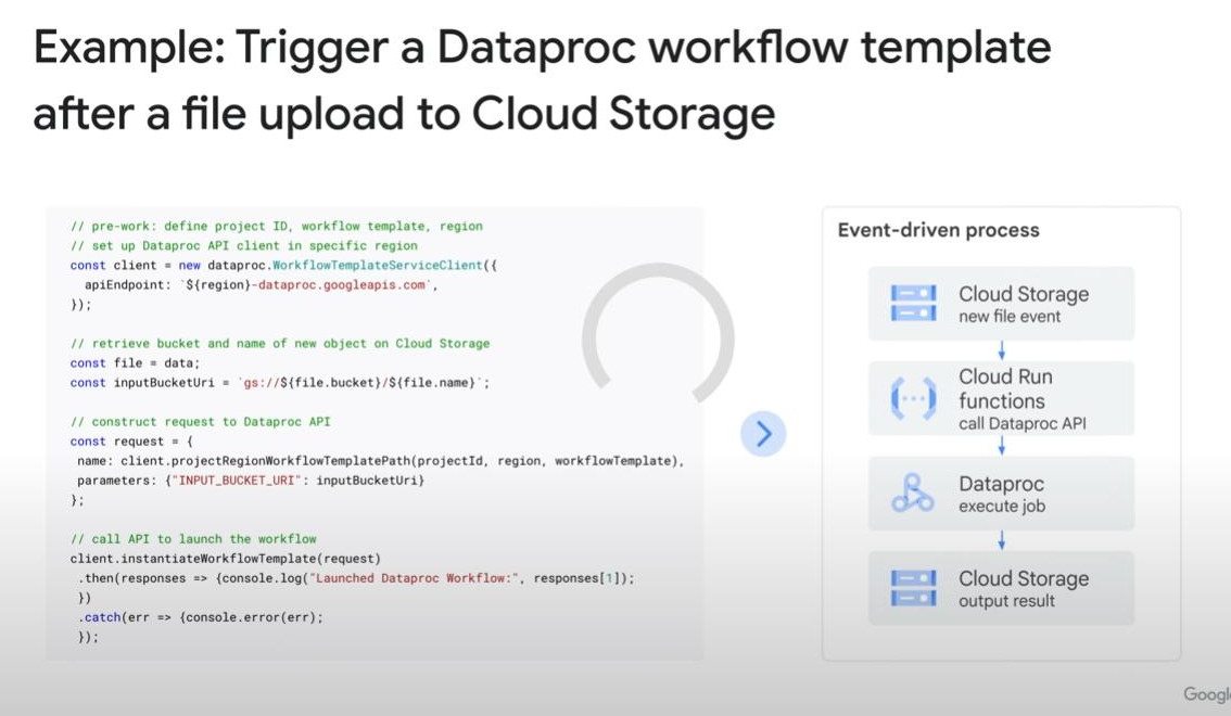
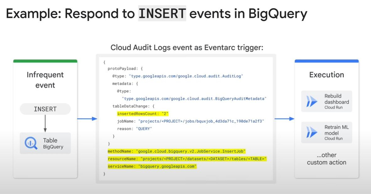
    • Eventarc is to build a unified event-driven architecture for loosely coupled services.

    

    • Summary:

    

12. Data engineer tasks.

    • Connect with Machine learning team:

      • How long does it take for a transaction to make it from raw data all the way into the data warehouse ?

      • Can you help us add more features (columns) of data into a certain dataset?

      • Key root: BigQuery-ML for directly creating a machine learning model inside BigQuery.

    • Connect with Data Analysts:

      • Our dashboards are slow, can you help us re-engineer our BI tables for better performance (faster) ?

      • Core key: BI-engine allows BigQuery to connect directly with Looker, Sheets, Partner-BI-tool. Both batch/streaming is available.

    • Connect with other data engineers:

      • We’re noticing high demand for your datasets – be sure your warehouse can scale for many users.

    • Data access and governance:

      • Data Catalog is a managed data discovery.

      • DLP (Data Loss Prevention): for guarding PII (Personal Identifiable Info). (redacting data at scale).

    • Build Product-ready pipeline:

      • Cloud Composer : is a managed Apache Airflow used to orchestrate production workflows.

13. Recap:

    

    

    

14. SLA (Servive Level Agreement):

    • An SLA (Service Level Agreement) in cloud service is a formal contract between a cloud service provider and a customer that defines the expected service quality, availability, and responsibilities of both parties. It ensures that the cloud provider meets specific performance standards and outlines the consequences if those standards are not met.

    

    • Multi-Region: 99.95% Availability means max downtime: ≈ 21.6 minutes per month.
    • Dual-Region: 99.95% Availability means max downtime: ≈ 21.6 minutes of downtime per month.
    • Single Region: 99.9% Availability means max downtime: ≈ 43.2 minutes per month.

15. Security with IAM: there are 2 main roles (customizable)

    • Bucket roles: bucket reader, bucker writer, bucket owner. Only IAM bucket role can modify access permission to a bucket. To create or delete a bucket is project-level roles.

    • Project roles: project viewer, project editor, owner role. Owner role could make users members of special groups like bucket-level roles.

    • Access list: it is different from IAM. It will be auto-enabled as creating a new bucket. You could give access permissons on only one file with either IAM or access list.

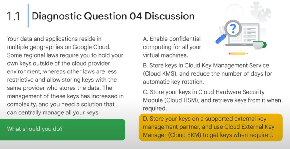
    • Encryption: we have 2 levels of encryptions with GMEK and KEK:

      • GMEK (Google-managed encryption key): data is first encrypted with GMEK.

      • KEK (key encryption key): GMEK is encrypted with KEK. KEK is rotated on scheduled and stored in Cloud KMS by default. But customers could store KEK in CMEK (customer-managed encryption key) or other third parties.

    • Client-side encryption: customers can encrypt before upload, then decrypt after download.

    • Lock types: Locking will deny any modification. We have bucket lock, Rentention Policy Lock, Object lock.

    • Gzip archives: it is data compression. With proper metadata, Cloud Storage could decompress the file as it is being served. Better is a lower cost for both uploading and storage.

    • Requester-pays-on-access: we can set a bucket with “requester-pays-on-access”. So requester will pay as they access the bucket. We only pay the storage.

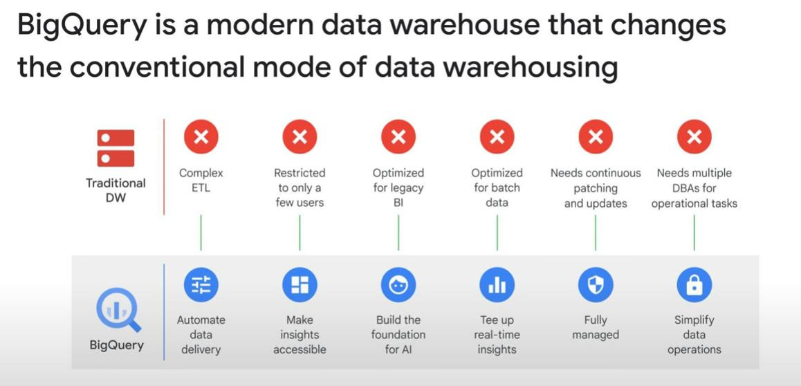
16. Data Warehouse:

    • BigQuery is a fully-managed service.

    • Data aging and expiration can be a cumbersome operation in traditional data warehouse => We have an expiration flag for a table in BigQuery.

    • BigQuery does not use Indexes on tables, we dont need to rebuild it.

    • Jupiter is to allows fast communication between compute and storage in BigQuery.

    • BigQuery tables are immutable and optimized for reading & appending, not updating. Reading Optimization means that most queries involve few columns, so it reads only few columns for the query.

    • BigQuery Slot is a combination of CPU, memory, and networking resources. Under the hood (behind the scenes), a BQ slot is a unit of computational capacity to execute SQL queries. But it is auto to calculate how many slots it need each query. Note: Slots can be different, each can have different CPU, memory or anything.

    • Query Service: is separated from the Query Storage, but we cannot see it.

    • The life of a BigQuery SQL query: result is a temporaty table and auto-stored for 24h in cache, if we re-run the same query, no charge occurs during the 24h. But when we store the result in a destination table, which is then a permanent table, so that we will get charged for permanent storage.

    • Cost of Storage & Cost of Query: They can be separated by Project, which is the boundary for billing. If project A contains permanent storage, then owner A will pay this storage. But if project B is used only to do SQL queries from the shared storage in project A, the owner B will only pay the cost of queries happending in the project B.

    • BigQuery Access Control: access control can be at level of datasets, tables, views, or columns.

    • Multi-zone VS multi-region: a dataset can be set to stored in a region, so it will be replicated to become multi-zone. Or, A dataset can be stored in multi-regioned.

    • View: it is a virtual table defined by a SQL query, you can share it externally without sharing the underlying data because we cannot export data from a view. View will always run everytime we run the query containing it. “Intermidiate table” is a basic solution but no auto update so it needs a “scheduled upate” service.

    • Materialized View: Bigquery will save “materialized view” permenantly and auto refreshed and updated with the contents of the source table. Materialized View can improve signigicantly ther performance of workloads. (note: storage cost will arise for “materialized view”). If we use “With clause” so many times, “Materialized view” will be a effective way to improve queries performance because “with clause” is not cached like “Materialized view”.

        CREATE OR REPLACE TABLE mydataset.typical_trip AS ...   --extra cost of storage and manual update
        CREATE VIEW my_dataset.active_users AS ...              --cost everytime running the view.
        CREATE MATERIALIZED VIEW my_dataset.monthly_sales AS ...    --extra cost of storage but auto update
    

    • Warning: “materialized view” depends on cache, but query can never be cached in following cases:

      • Queries are never cached if they exhibit non-deterministic functions (CURRENT_TIMESTAMP() or RAND())
      • If the table or view being queried has changed (even if the columns/rows of interest to the query are unchanged)
      • If the table is associated with a streaming buffer (even if there are no new rows)
      • If the query uses DML statements (INSERT, UPDATE, DELETE, and MERGE), or queries external data sources.

    • If you find yourself using a WITH clause, view, or a subquery often, one way to potentially improve performance is to store the result into a intermidiate table (or materialized view).

    • Authorize Views: an “authorize view” allows to share query results to particular users or groups without giving them access to the underlying source data.

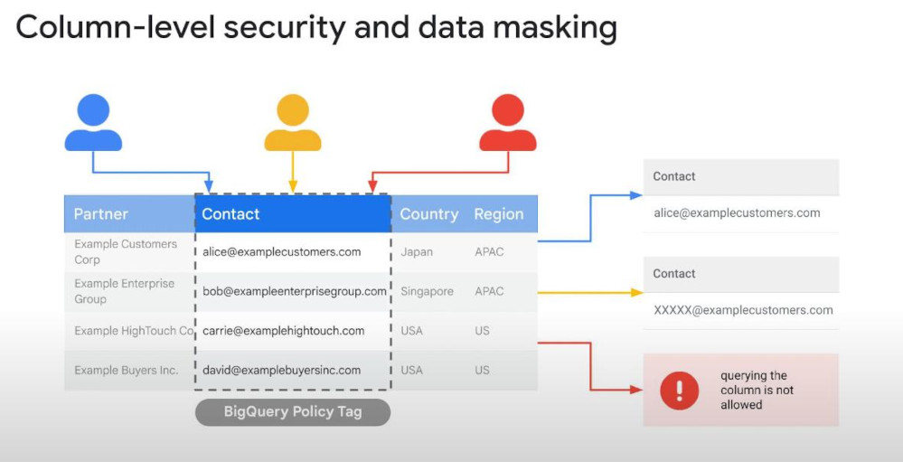
    • Column-level security: we can assign “Policy Tag” to a column, then assign users or groups to it, then these users will be able to see the column’s content.

    

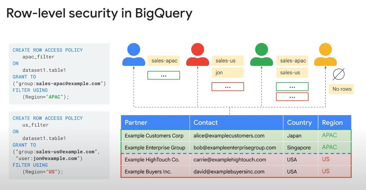
    • Row-level security: look at the query in the image below, this security acts as a filter to show/hide certain rows depending on users/groups allowed or not.

    

    • BigQuery Transfer Service: help us build and manage the data warehouse with “connectors”, “transformation templates” and “scheduling”. “BTS” is also used to move data between regions.

    • Automation: we can automate the execution of queries based on a schedule. Scheduled queries must be standard SQL. Within 7 days, you can easily revert changes without requesting a recovery from backups.

    • DML Statement (Data Manipulation Language): used to change data within tables. BigQuery supports “standard DML statements” like INSERT, UPDATE, DELETE, & MERGE.

    • DDL Statement (Data Definition Language): used to modify structure of a databas, like tables, indexes, schema (CREATE, ALTER, DROP, TRUNCATE). It is “CREATE OR REPLACE TABLE” & “CREATE TABLE IF NOT EXISTS” in BQ.

    • UDFs - (User defined function): BigQuery supports user-defined functions in SQL. We can create a function direcly like image below. We can store UDFs persistently as an object in the database source (GitHub), then share it.

    

    • Sometimes or All the times, we need to explore all warehouse tables in a very short time, of course we could use the BQ UI to do that, but it follows one by one rule, meaning it does not combine all info into a page. That’s why we need a query to do that, so we could know, number of rows, volume, created date, last modified date, type of all tables (table or view) of a dataset.

    • How to check if a table schema changes in our project or dataset?

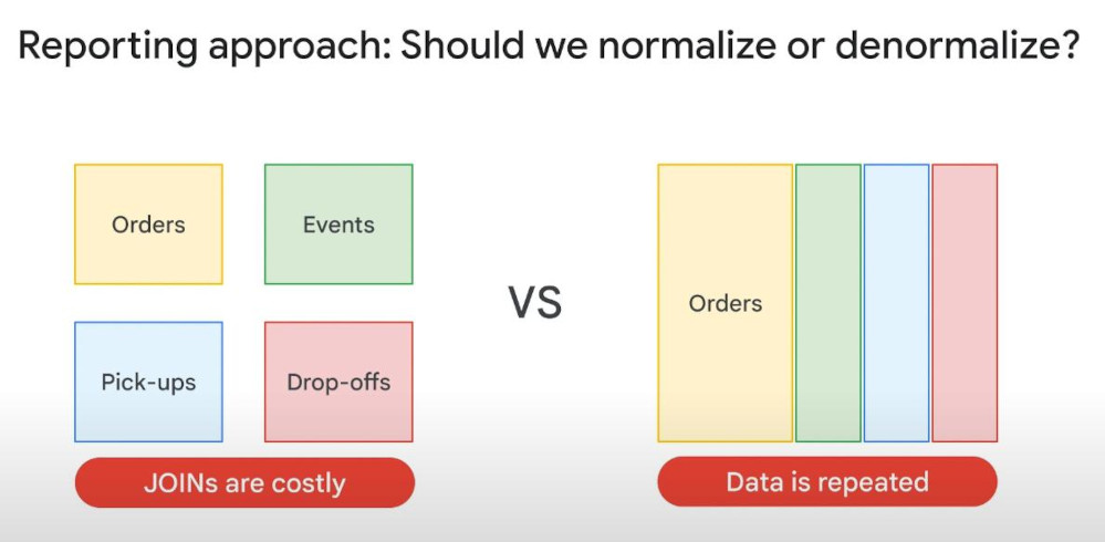
    • Normalized >< Denormalized Form: Transactional databases often use normal form. Normalization increases the orderliness of the data, which is then useful for saving space. But data warehouse is different, it implies denormalized form. Denormalization allows duplicate columns, which will take more storage but make queries more efficient. Queries can be processed in parallel using columnar processing. Specifically, Denormalization will enable BigQuery to distribute processing among slots.

    

    • Warning: Some denormalization with flatenned table can cause shuffling (back & forth) between network and system, that is slow. Solution is to combine denormalization with nested and repeated data like image below, helping each whole order is co-located and eliminate shuffling. (relational database turns out to be fit for nested and repeated data denormalization.)

    

    • GOJek problem: GOJek (Indonesia) processes over 13PB/month (10^9 MB) to support business decisions. They have many orders daily, what should they do when they need order reports monthly. One order is a ride with a pickup/drop_off destination, ride confirmation event, route. Now Both normalization and denormalization is not effective because of either _many JOINs or data repeated

    

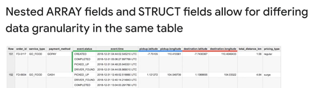
    • Solution: We need nested columns (arrays). Now we have 2 new type STRUCT and ARRAY, which is typical POINT in their names. But they are different data types in SQL. Struct is a type of record at schema, Array is a repeated mode, array of strings, array of floats, …Array can be part of regular field or nested fields inside a Struct. (BigQuery natively supports arrays, Array values must share a same data type, Arrays are called REPEATED fields in BigQuery)

    • If our database shape is STAR schema, SNOWFLAKE and THIRD NORMAL FORM.

    

    • RECAPs: (the crossover is 10GB, since then, JOIN impact becomes significant)

      • Instead of JOINs, take advantages of nested and repeated fields in denormalized tables.
      • Keep a dimension table smaller than 10GB normalized, if they go usually with UPDATE or DELETE operations.
      • Denormalize a dimension table larger than 10GB, unless data manipulation cost outweigh benefits of optimal queries.

17. Optimize with Partitioning and Clustering:

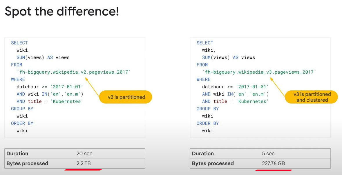
    • Both partitioning and Clustering help reducing the cost and amount of data read by partitioning your tables.

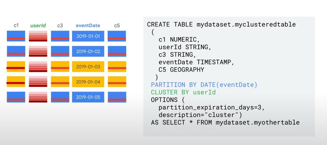
    • Shard: if we partition a table by the event DATE column, BigQuery will then change its internal storage so the DATEs are stored in seperate shards. Now, if we filter with “WHERE date=’2017-01-03’” with partitinoned field DATE on the left side, BigQuery will only scan rows corresponding with the shard “2017-01-03”, not the full table. This lead a dramatic cost and time saving, but a litle more metadata will be managed of course.

    • There are 3 ways at different stages while creating a new table (exclude BQ_SQL):

      - INGESTION TIME : bq query --destination_table mydataset.mytable --time_partitioning_type=DAY
      
      - A TIMESTAMP TYPE COLUMN: bq mk --table --schema a:STRING, tm:TIMESTAMP --time_partitioning_field tm
      
      - Integer Type column:
          bq mk --table --schema "customer_id:integer, value:integer" \
              --range_partitioning=customer_id,0,100,10 mydataset.mytable
      

    • What is CLUSTERING ?: _BigQuery will auto SORT values in the clustered column, “these sorted values” will then be used to organise the data into many “sorted BLOCKs” in its storage, also reducing scans of un_necessary data, particularly for queries that aggregate data based on CLUSTERED column because the sorted BLOCKs co-locate rows with similar values. If we cluster multi-columns (4 or more) the order of columns is important because only the first column is sorted truly. We cannot cluster a nested column. _.

    • Notice: In streaming tables, we need continuous re-clustering, BigQuery will auto handle that underground.

    • We can set partitioning and clusterning at creation time:

    

    #standardSQL
    CREATE OR REPLACE TABLE ecommerce.partition_by_day
    PARTITION BY date_formatted
    OPTIONS(
        description="a table partitioned by date"
    ) AS
        ---source table here---
        SELECT DISTINCT
            PARSE_DATE("%Y%m%d", date) AS date_formatted,
            fullvisitorId
        FROM `data-to-insights.ecommerce.all_sessions_raw`
    

    • What if PARTITIONING + CLUSTERING ?: although “partitioning benefits” can be defined before running a query, “cluctering benefits” cannot. However, their combination is usually better. When they combine, each partition is clustered based on the values on the clustering columns. KEEP IN MIND: if we want to cluster a non-partitioned table, we should add more a column named ‘fake_date’ of type DATE, and all the values is NULL, BigQuery will treat it as single SHARD of partitioning.

    

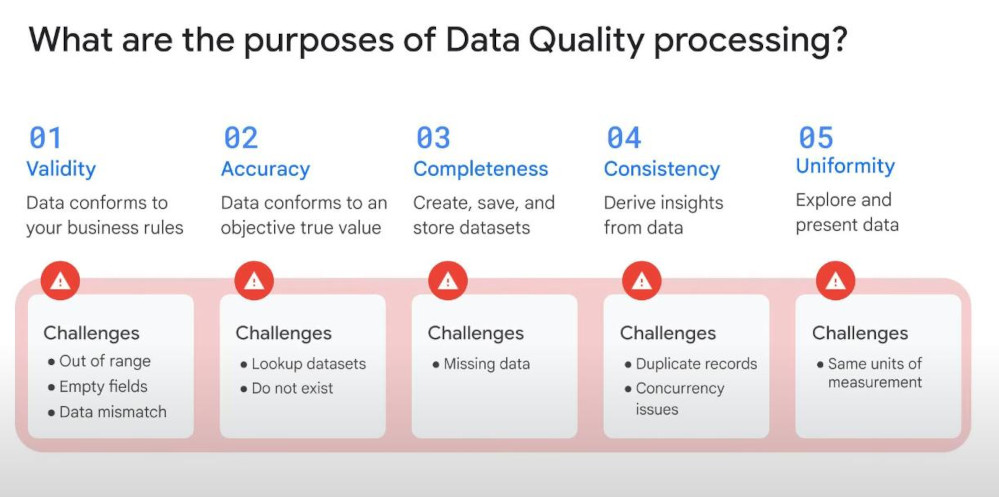
18. Data Quality or “VACCU” :

    • Validity : it conforms business rules (đúng quy cách, hợp lệ)
    • Accuracy : objectiveness (khách quan)
    • Completeness : complete (đầy đủ)
    • Consitency : consistent (nhất quán)

    • Uniformity : uniform (đồng nhất, đồng dạng hay đơn vị)

    • Data Quality issues can be fixed by ‘BigQuery View’ through ELT pipeline.

    

19. Cloud Logging and Cloud Monitoring: both can help customize LOGs, monitor jobs and resources. Below is some examples:

    • Error that caused Spark job failure: just look at the logs generated by Spark executioners. (if the job was submitted to primary node using SSH, logs cannot be seen.). The logs output is stored on storage bucket of the Dataproc cluster,

    • stdout VS stderr: stdout is usually successful messages, stderr is for errors happening.

    • Cloud Logging: contain Yarn, which collects all logs by default. Yarn is available in a Dataproc Cluster.

    • If our clusters or Dataproc jobs have labels, logs can be easily found by these labels.

    • Cloud Monitoring: help monitoring the cluster’s CPU, disk, network usage and Yarn resources. We even can customize dashboard to show these metrics.

20. Cost consideration:

    • slots are units of processing that help clients to manage resources consumption and costs. Bigquery will automatically calculate how many slots are required by each query denpendent on size and complexity as running.
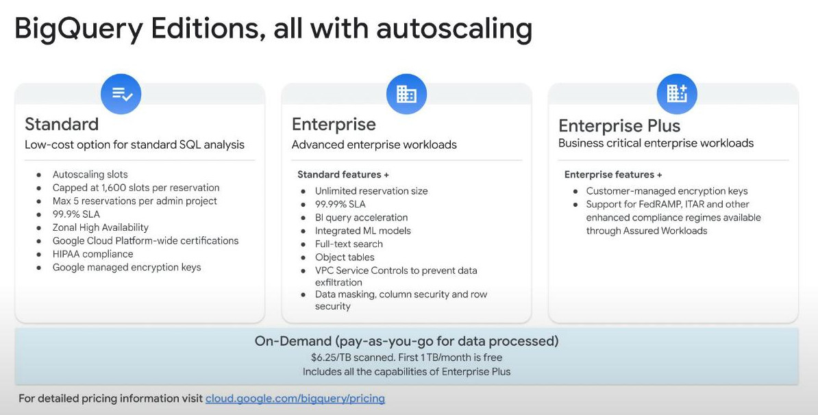
    • Bigquery Editions: there are 3 edition tiers (3 nấc, 3 bậc). All options are auto-scalabitity. The last thing is an optional feature to reduce storage cost with compressed storage.
      1. Standard Tier: entry-level, low-cost option for standard SQL analysis that is suitable for all requirement of basic workloads.
      2. Enterprise Tier: offers a broad range of analytics features for workloads that demand higher capability, flexibility, and reliability..
      3. Enterprise plus Tier: designed for advanced features, mission-critical workloads that require multi-region support, cross-cloud analytics, advanced security and regulatory compliance.
         • Besides, there is also to “mix and match” edition based on individual workload demands.
         • In addition to the 3 pricing tiers, there is an on-demand pricing option that allows clients to pay for data they process. (6.25$/TB ~ 1k GB).

    

    • Despite slot auto-scalability, we need set maximum size and an optional baseline for reservation. It is a serverless architecture. Slots are added or removed on-demand, we only pay the slots they consumed.

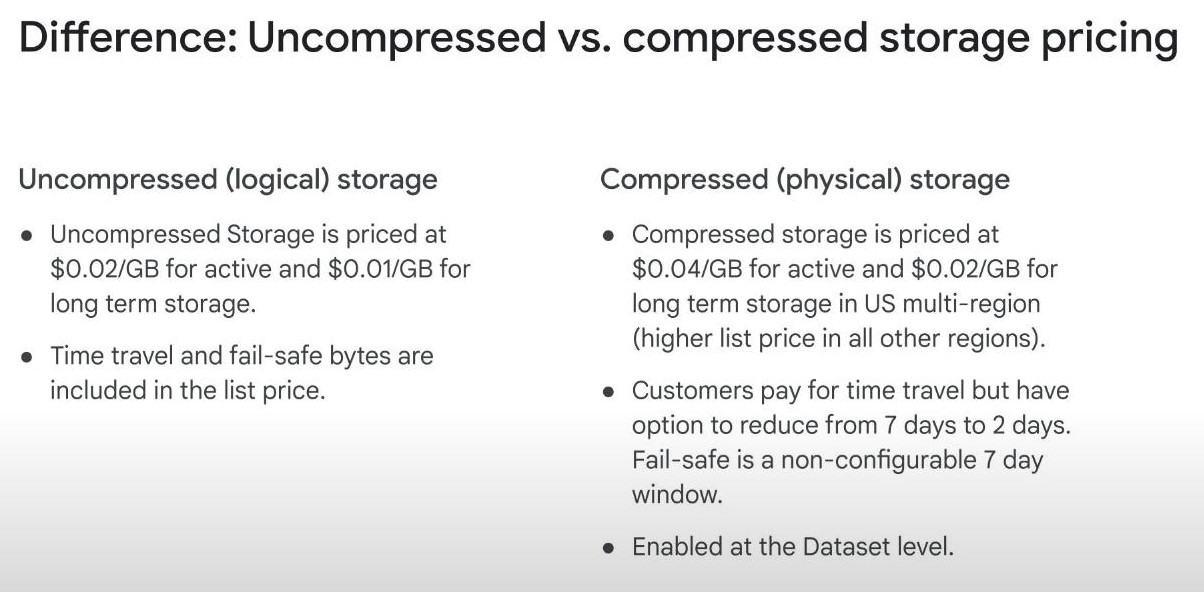
    • Compressed Storage with Exabeam: sometimes we have to re-balance costs between storage and compute. Now, exabeam help us solve it very well. Note that, uncompressed storage is more expensive 2 times than compressed storage.

    

    • Time travel vs Snap-shot Time Travel in cloud storage (BigQuery) refers to the ability to access previous versions of data at a specific point in time. These versions are kept for a limited time (up to 7 days in BigQuery). We can reduce it to 2 days to reduce storage cost. For longer time backup, we have to create snapshot to store the old table verion permanently. (Note: “time travel” is auto-updated but snapshot is not).

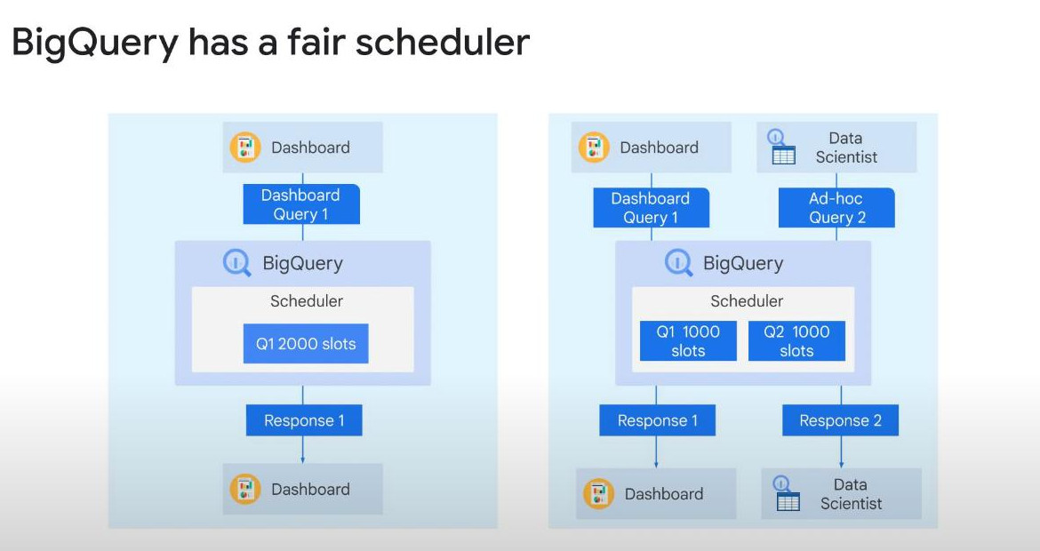
    --change time travel from 7(default) to 3: (0 = disable time travel)
        ALTER SCHEMA my_dataset
        SET OPTIONS(time_travel_retention_days = 3);
    
    --restore data of yesterday (using Time travel).
        SELECT * FROM my_table
        FOR SYSTEM TIME AS OF TIMESTAMP_SUB(CURRENT_TIMESTAMP(), INTERVAL 1 DAY);
    
    --create a snapshot for long-term backup.
        CREATE SNAPSHOT TABLE my_project.my_dataset.snapshot_table
        CLONE my_project.my_dataset.original_table;
    

    • 2000 slots = 50 complex queries: Because Bigquery does not allow us to set slots prioritized for a specific query, its auto-scalability assures fair resource allocated among all queries. So, estimating the right number of slots from beginning is critical to ensuring query performance. Bigquery will stop any queries that run over 6 hours. For example, if we execute only one query, Bigquery will use all 2000 slots for it, but when we execute 2 queries concurrently, each query will get half of total slots available, in this case 1000 slots each. This subdividing of compute resources will continue happens as more queries are executed. This is a long way of saying, it’s unlikely for one heavy resource query will overpower the system and steal resources from other running queries.

    

    • Unfair Division at project level: we can set up a unfair hierarchical reservation in case we know that one project require somewhat lower resource than other projects. We can set a maximum number of slots for it, then it can never use over this maximum.

21. Dataflow:

    • Beam Portability framework:

      • Original vision is to allow users to write data pipelines in the programming language of their choice and run it on the engine of their choice. Optional languages are Python, Java, Go, SQL.
      • Allows moving pipelines from premise server to Dataflow.
      • Portability API is an inter-operability layer enables us to use the language of choice with the engine of choice.

    • Dataflow Runner v2:

      • Portability (Apache Beam) helps us build a data pipeline that will be uploaded and executed by various runners. Some users prefer to run their pipelines on-premises or in multi-cloud environments (a multi-serviced combinations of AWS, Cloud, and Azure). But in this section, the pipeline will be uploaded and executed onto Dataflow by a runner called “Dataflow Runner”. It is like a translator between Portability and Dataflow instance.

      • Dataflow itself can operate alone without using Portability, for example “SQL-based data processing”. However, we will lose most of useful features supported by Portability as mentioned in “Beam Portability”.

      • Runner are packaged together with “Dataflow Shuffle” service and “the streaming engine”.

      • Most of times, “Runner v2” is auto-enabled, but we can use it at runtime by using flag (formed with “–“) in the command line CLI:

          --experiments=use_runner_v2
          --experiments=disable_runner_v2
      

    • Container on-cloud:

      • The Beam SDK “runtime environment” can be containerized with Docker. (Note: containerization is a way to isolate oneself from other runtime systems). So, each user operation has its own separate environemnt in which to execute.
      • A default environment supported by SDKs can be further customized.

      • Because of “available containers” in Cloud service, we can benefit from ahead-of-time installation that includes “arbitrary dependencies”. Even “further customization” is possible.

      • To run your pipelines on custom containers, Beam SDK v2.25 or later is required.

      • To create a custom container image, specify the Beam SDK as a parent image starting with “FROM” as below in Dockerfile, then add your own customization.

      

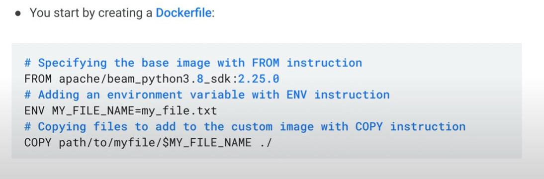
      • After creating the Dockerfile, we have to build the image, push it to the container registry on Cloud (gcr.io) that is an address where container images are stored and managed.

      

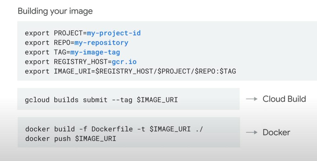
      • Finally, launch Dataflow pipelines by referencing regular parameters including the location of your container image.

      

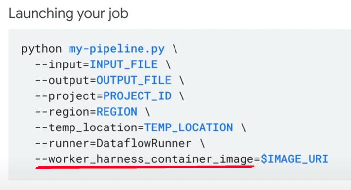
    • Cross-language Transform of Beam Portability:

      • With a language-agnostic representation of pipelines and the possibility to specify the environment for each operaion, we are no longer limited to a single language in a given pipeline.
      • Portability (not its framework) allows us to run a multi-language pipeline that leverage the respective benefits of different languages. In specific, we can write a Python pipeline while using I/O connectors that were only available in Java. Or we can even use a Tensorflow extended block of code for a Machine Learning model in a Java pipeline.
      • The code below is a part of a Python streaming pipeline. The transform method “ReadFromKafka” is imported from the “apache_beam.io.kafka” module that is Java-based.

      

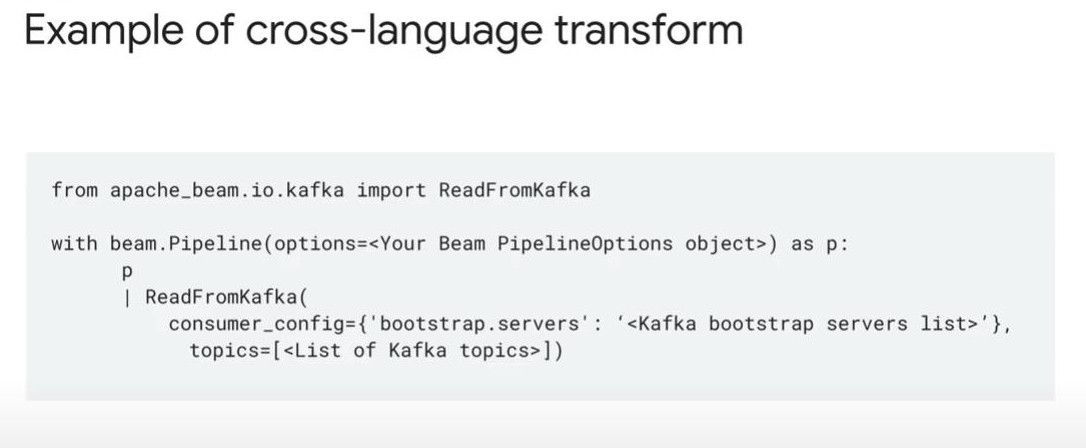
      • Under the hood, to use a Java transform method in a Python dataflow pipeline, the Python Beam SDK has to create and inject appropriate Java pipeline fragments to the Python pipeline, then it has to download the necessary Java dependencies to execute the Java transform. That means, at runtime, VM workers must run both Java and Python code simultaneously.

    • Separate compute and storage: we have 4 sections.

      1. Dataflow:

         • Fully-managed and auto-configured.
         • Automatically optimize the graphical pipeline by fusing operations effectively, and by not waiting for a previous step to finish before starting a new one. (in parallel)
         • Autoscaling happens step by step in the middle of a pipeline job, as a job needs more resources, it will recieve them automatically without any manual intervention. We dont pay for VMs that aren’t being used. Dataflow will turn down the workers as the job demand decreases.
         • With intelligent watermarking to improve latency, aggregation functions (SUM and COUNT) remain correct even if the input sends duplicate records. It dynamically adjusts watermarks based on the characteristics of incoming data. So, watermark is an estimate, not a fixed threshold in the timeline of streaming.

      2. Dataflow Shuffle

         • It’s important to note that Dataflow Shuffle is a foundational operations behind transforms such as GroupByKey, CoGroupByKey, and Combine. Shuffle refers to partition or group data by key in a scalable, efficient, and fault-tolerant manner. There are 3 types:

         • Default Dataflow Shuffle runs entirely on worker VMs and consumes worker CPUs, memory, and persistent disk storage.

         • Service-based Dataflow Shuffle is only for batch pipeline and runs entirely on Dataflow service backend using Cloud Storage instead of woker VMs. So, we’ll benefit from a reduction in consumed CPU, memory and persistent disk storage resources on worker VMs, meaning worker VMs no longer hold any shuffled data, resulting in essential resilience where if one worker is broken accidentally, it will not cause the entire pipeline to fail with it. Service-based Shuffle certainly has better fault-tolerance.

         • Another type is Streaming Shuffle implemented within the dataflow streaming engine.

      3. Dataflow Streaming engine

         • offloads the window state storage from worker VMs disk to a backend service.

         • Luckily, no code changes are required with Dataflow Streaming engine. Worker nodes remain running your user code, implementing data transform, and transparently communicate with the streaming engine to manage state (windowing, aggregations).

         • n1-standard-2 is a smaller but faster worker machine type that runs behind the Dataflow Streaming Engine, making it more responsive to variations in incoming data volumne.

      4. Flexible resource scheduling (FlexRS)

         • Let’s talk about “Flexible resource scheduling” or in short “FlexRS”.

         • FlexRS helps us reduce the cost on batch pipelines because of:

           • Advance scheduling
           • Service-based Dataflow Shuffle.
           • Mix of pre-emptible and standard VMs (that are cheap but can be stopped anytime).

         • When we submit a FlexRS job, Dataflow will place it into a queue, and submits it for execution within 6 hours from creation. This makes FlexRS suitable for workloads that are not time-critical such as daily or weekly jobs that can be completed within a certain time window.

         • Although FlexRs jobs are placed in a queue but Dataflow will immediately perform an early validation run to verify execution parameters, configurations, quotas and permissions. In case of failure, errors will be reported immediately.

22. IAM roles, Quotas, and Permission: (Omar Ismail):

    • Let’s start with some questions like:

      • How IAM provide access to different Dataflow resources. Or What happens as our Beam code is submitted?
      • When the pipeline is submitted, it is sent to 2 places:
      • The SDK uploads the Beam code to Cloud Storage and sends it to the Dataflow service.
      • The Dataflow service does a few things:
        • validates and optimize the pipeline.
        • creates the compute VMs required to run the code.
        • deploys the code to the VMs.
        • Gather monitoring information for display.
      • When all those above jobs are done, the VMs will start running the code.

    • At each of stages mentioned above, IAM plays a role in determining whether to continue the process.

    • 3 Credentials to determine whether a dataflow job can be launched.

      1. “User role” credential: whether a person is allowed to submit the code is determined by the IAM role assigned to their account. Your account is represented by your email address. Three user roles can be assigned to each user. Each role is made up of a set of permissions:

         • Dataflow viewer role: users, who is assigned with this role, can only view the Dataflow jobs, but cannot submit, update, or cancel jobs.
         • Dataflow developer role: suitable for person whoes job is to manage the pipeline. Users, having this role, might only view and cancel jobs that are currently running, but they cannot create/edit a new job beacause the role doesn’t have permission to stage files into a storage bucket and view the Compute Engine Quota.
         • Dataflow admin role: it is a minimum set of permissions that allow both creating and managing Dataflow jobs. Permissions include interacting with Dataflow jobs, staging files in an existing cloud storage bucket, and view the Compute Engine quota.

      2. “Dataflow service account” credential:

         • It is used to interact between projects such as checking project quota, creating worker instances, managing Dataflow jobs at run time:
         • When we run a Dataflow pipeline, Dataflow will use a service account “service-PROJECTNUMBER@dataflow-service-producer-prod.iam.gserviceaccount.com”, which is automatically created when Dataflow API is enabled. This service account is assigned the “Dataflow service agent role”, which grants necessary permissions to run a Dataflow job.
         • In the following diagram, the interactions of Dataflow service account is at the “HERE” on the medium right between the project and Dataflow

         

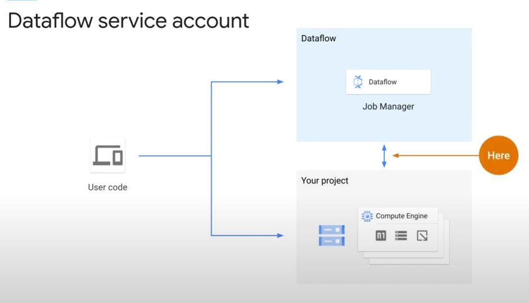
      3. “Controller service account” credential:

         • It is assigned to the Compute Engine VMs to run a Dataflow pipeline.

         • By default, worker nodes use the project’s “Compute Engine default Service Account” as the “Controller Service Account” in pattern PROJECTNUMBER-compute@developer.gserviceaccount.com, which is automatically created when we enable the Compute Engine API.

         • Note: the “Compute Engine default service account” has a broad access to project’s resources, which makes easy to get started with Dataflow. However, for production workflow, it is recommended to create “a new service account” with only the roles and permissions in need. At a minimum, this new service account should have “Dataflow worker role” and can be used with a “–service_account_email” flag when launching a Dataflow pipeline.

         • Besides, we might have to add additional roles to access different Google Cloud resources. For reading Bigquery, your service account must also have a “Bigquery data viewer” role. “HERE” is the location of the Controller service account’s interactions.

         

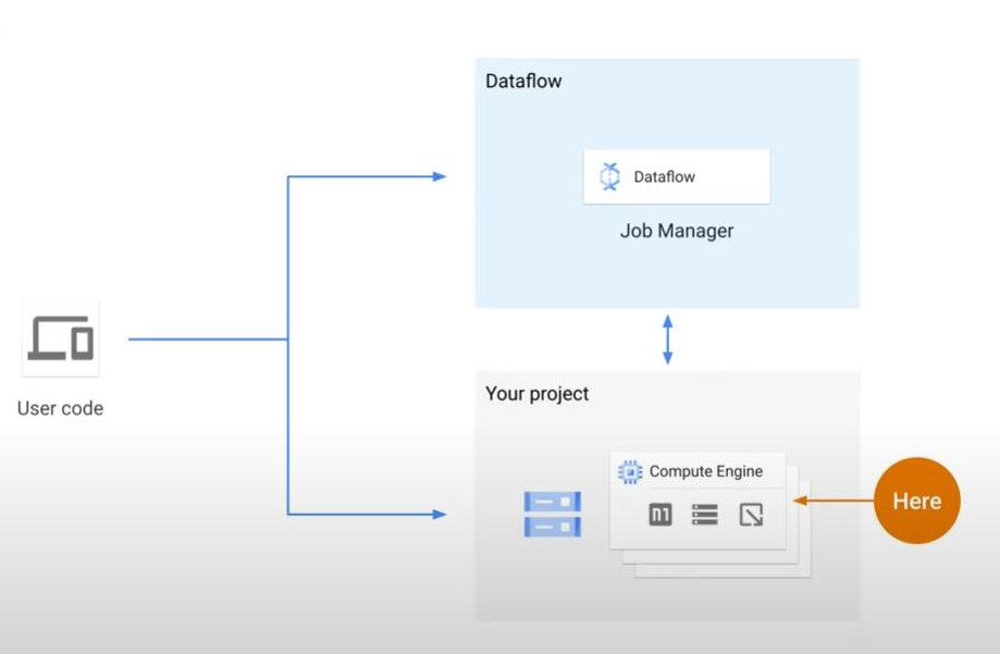
    • Quotas: what does it mean?

      • CPU quota is the total number of virtual CPUs across all of your VM instances in a region or zone. Any Google Cloud service that creates a Compute Engine VM as Dataproc, AI notebooks, or Dataflow consumes this CPU quota. “CPU quota” can seen in the “IAM quota page”.So, what it the CPU your dataflow job needs over the CPU quota? => error “CPU quota has been exceeded” will be reported.

        • n1-standard-1 (VM type) : 1 VM has only one CPU.
        • n1-standard-8 (VM type) : 1 VM has 8 CPUs.

      • IP quota: refers to the total number of in-use IP addresses in each region. This IP quota limits the number of VMs that can be launched with an external(public) IP address for each region in your project. The IP quota is shared across all Google Cloud products that create VMs with external IP addresses (public IP):

        • There are 2 types IP, internal IP and external IPs. The first is for internal communication within Google Cloud. The second is to access external services outside Google Cloud.
        • By default, when launching a Dataflow job, the VM is assigned an external IP address. This is required if the job needs to access external APIs or services outside Google Cloud. However, if the Dataflow job doesn’t require external services, we can manually re-configure it to use only internal IPs. This helps save costs and conserve the “IP quota”.

      • Persistent Disk quota (PD quota): we can choose the disk type (HDD or SDD). By default, it will be HDD disk.

        • To select SDD, use the flag –worker_disk_type at CLI in Python:

        python3 -m apache_beam.xyz \
        --worker_disk_type compute.googleapis.com/projects/$PROJECT/zones/$ZONE/diskTypes/pd-ssd (SSD)
        
        IN JAVA: gradle clean execute -DmainClass=org.apache.beam.xyz \
        --workerDiskType=compute.googleapis.com/projects/$PROJECT/zones/$ZONE/diskTypes/pd-standard (HDD)
        

        • For batch pipeline: when we lauch a pipeline, the ratio VM to PD is 1:1 (1 to 1)
        • For batch pipeline: for jobs running Shuffle on worker VMs, the default size of each persistent disk (PD) is 250GB.

        • For batch pipeline: for service-based Shuffle, the default PD size is only 25GB (recall that service-base Shuffle moves the shuffling operations out of worker VMs to the Dataflow backend service, which is why the attached PD size is smaller).

        • We can use *disk_size_gb flag* in Python to overwrite the default persistent disk (PD) for batch pipelines. (*diskSizeGb flag in Java*)

        • For streaming Pipeline: PD are allocated from a fixed pool. Each worker must have at least one attached PD, with a maximum limit is 15 PDs per worker VM. Similar to “batch jobs”, “streaming jobs” can be run either on worker VMs or utilize the Dataflow Streaming Engine. When we run on the Dataflow Streaming Engine, which offloads some operations from worker VMs into the Dataflow’s service backend. For the streaming case, the default PD size on each worker VM is 400GB and on Streaming Engine is 30GB. The flag is used to overwrite it is the same as batch pipeline.

        • It’s important to note that the amount of PDs allocated in a streaming pipeline can auto-scale to the value set in the flag max_num_workers. This flag is required when running on the worker VMs and its value cannot exceed 1000. For the Dataflow Streaming Engine, the flag is optional with default value of 100.

23. SECURITY: “How many ways to enhance security while running Dataflow? or What is security?” There are 4 security features in this module:

    1. Data Locality: it ensures all data and metadata stay in one region. Because it affects who can access the data, where it is physically stored, and what laws govern its protection.

       • As we discussed in the IAM module, the Dataflow Service Account communicates between our project resources and the Dataflow backend. The Dataflow backend exists in a few regions across the globe and can be different from the region where our worker VMs run.

       • What metadata is transfered between our project and the “regional endpoint” (the Dataflow backend). Worker VMs, which take actions of some “health checks”, request a “work item” and the regional endpoint (backend region) responds with a “work item”, the “worker item status” and “autoscaling events”. (item = task)”

       • Unexpected events” are also transfered to the “regional endpoint” like *unhandled exceptions in user code, jobs that failed because of lacking permissions, worker item failures, and errors from another related system such as Compute Engine. These items are available and visible in the Dataflow UI along with other info such as pipeline parameter values, job name, job ID and *start time*.

       • Regional endpoint: “us-central1” is a regional endpoint. Why do we have to specify a reginal endpoint?

         • Definition: A regional endpoint is a service-specific URL that directs requests to a specific geographic region in a cloud provider’s infrastructure. It ensures that workloads are executed within a designated region for lower latency, network transfer cost, compliance, and high availability.

         • Firstly to support “project security” and “compliance needs”. For ex, in some countries, a regional regulatory rule mandates that data of banking systems does not leave the country of operation. This rule can be met with a specific “regional endpoint”.

         • Network egress will not be charged if our pipeline sources, syncs, and staging locations are all in the same region.

       • –region VS –worker_zone VS –worker_region: if we have no “zone preference”, just specify the flag ”–region” only. In this case, the regional endpoint will automatically select the best zone based on “available capacity”. Otherwise, use –worker_zone $WORKER_ZONE to specify a zone.

       python3 -m apache_beam.xyz --region $REGION
       gradle clean execute -DmainClass=org.apache.beam.xyz --region=$REGION
       

       • Note: in case, we want worker processing to occur in a region that does not have “a Dataflow regional endpoint”, use both –region and –workerregion flags. the region flag is to specify the supported endpoint, that is _closest to the region where the workers run in, and –workerregion for the region where the workers run in. This case can happen because sometimes data is stored in a different region that does not have a Dataflow regional endpoint (_so we wanna set the –region close to it) OR the default region has limited resources or quota.

       • Keep in mind: Even if no regional endpoint exists in the region we want our data to be stored, only metadata is transfered, the application data remains in that region.

    2. Shared VPC (virtual private cloud = a network): Another feature we can use with Dataflow is “shared VPC”, which provides routing, firewall rules, and connectivity options.

       • Host project: Dataflow can run in networks that are either in the same project or in a separate project called (“the host project”).

       • When a network exists in a host project, say the networking setup is “shared VPC”.

       • “A Shared VPC” let organization admins delegate administrative responsibilities (such as creating and managing instances) to others while maintaining centralized control over network resources like subnets, routes and firewalls.

       • When we should set “same VPC”?:

         • Definition: A VPC can span(extend) multiple regions, allowing resources in different locations to communicate. A Subnet is associated to only one region within the network.
         • A custom network refers to manually configure some regions, and some subnets.
         • When setting the number of VMs to use, remember to have enough IP addresses available. For ex, we have a subnet “/29” without any VMs running on it, the maximum number of Dataflow workers that we can launch is only 4. We should choose subnet “/27” with 28 availabe IPs in case of heavy-load Dataflow jobs. (in following image).

         

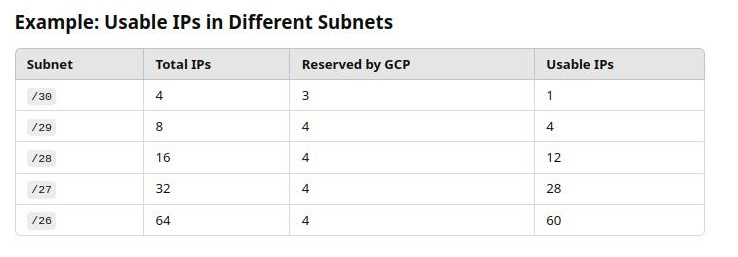
         • Note: the Dataflow service account needs “Compute Network User” role in the host project (either project-level or subnet-level).

         • Use –network or –subnetwork flag.

         ## project_level "Compute Network User"
         python3 -m apache.beam.xyz ... --network default
         
         ## subnet_level "Compute Network User"
         gradle clear execute -DmainClass=org.apache.beam.xyz \
         --subnetwork=https:.../compute/v1/projects/$PROJECT_ID/regions/$REGION/subnetworks/$SUBNET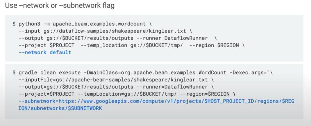
         

         

    3. Private IPs: Another security we can use is to disable external IP usage, blocking users to access the internet.

       • Dataflow service can assign workers with both public and private IP addresses. When we turn off public IP addresses, the Dataflow pipelines access resources only in the following places:

         • Another instance in the same VPC network.
         • A shared VPC network.
         • A network with VPC network peering enabled.

       • If our pipeline is communicating with other Google Services and APIs and is in a custom network, the Private Google Access must be enabled for the subnetwork your workers will be launched. If the Private Google Access is disabled and there is no other way of reaching the internet (like Cloud NAT), VM instances can no longer reach Google services or APIs.

       • To user private IPs only, we have to add 2 flags: –network or –subnetwork, and –nouse_public_ips (_use internal(private) IPs only)

       python3 -m apache.beam.xyz
        --subnetwork regions/$REGION/subnetworks/$SUBNETWORK
        --no_use_public_ips
       
       graddle clean execute --DmainClass=org.apache.beam.xyz \
        --subnetwork=regions/$REGION/subnetworks/$SUBNETWORK \
        --usePublicIps=false
       

    4. CMEK stands for Customer Managed Enscrytion Key

       • Where data is stored:

         • Cloud storage bucket: is used to store binary files containing pipeline code. It is also used a staging areas to temporarily store export or import data between different services.

         • Persistent Disk (attched at workers): used for disk-based(default) shuffle and streaming state storage.

         • If a batch job is using Dataflow shuffle (service-based shuffle), the backend stores the “batch pipeline state” during execution. This means intermediate results, shuffle data, and execution progress are stored outside of worker nodes.

         • If a job is using Dataflow Streaming Engine, instead of workers, the backend will store the streaming pipeline state during execution. Dataflow Streaming Engine moves streaming state management and shuffle operations to a Dataflow backend, rather than relying on worker VMs’ memory or disk.

       • By default, when data is stored in any of those above locations, Google Cloud automatically encrypts all data at rest using Google-managed keys. CMEK gives us control over this encryption by allowing us to use our own keys stored in Google Cloud KMS (keys managenent sys). Because CMEK is supported across multiple Cloud storage services, we can use CMEK in any of data storage locations mentioned.

       • When a pipeline starts, data is loaded into workers memory. Data keys (ID, timestamp) used in key-based operations, such windowing, grouping and joining, and those keys, which were encrypted using CMEK, will be decrypted before being used in the pipeline execution for functioning correctly. For additional layer of secutiry, we can hash or transform the keys before encryption.

       • Job metadata is ecrypted with Google encryption. Job metadata includes the following:

         • User data
         • Job name
         • Job parameter values
         • Pipeline graphs
         • System-generated data like IP addresses and job IDs

       • Using CMEK requires both the “Dataflow service account” and the “Controller Agent Service account” to have the Cloud KMS Cryptokey Encrypter/Decrypter role.

       • We need 2 flags to use CMEK: –temp_location & –dataflow_kms_key.

       python3 -m apache.beam.xyz \
       --tem_location gs://$BUCKET/tmp \
       --dataflow_kms_key projects/$PROJECT/locations/$REGION/keyRings/$KEY_RING/cryptoKeys/$KEY
       
       graddle clean execute -DmainClass=org.apache.beam.xyz \
       --temLocation=gs://$BUCKET/tmp \
       --dataflowKmsKey=projects/$PROJECT/locations/$REGION/keyRings/$KEY_RING/cryptoKeys/$KEY
       

       • Note: when we use CMEK for a Dataflow job, the region for our key and the region where Dataflow job runs must be the same. Global or multi-regional keys will not work. The bucket selected to temporarily store data must also be in the same region as the key.

24. Develop Dataflow Pipelines:

    • There are 3 ways to launch a Dataflow pipeline:

      1. Launching a template using Create Job Wizard in Cloud Console. No need to write code with this option. All we have to do is to select a template from a drop-down menu, fill out a few fields, and the job will be deployed. We’ll cover this workflow briefly in the Building Batch Pipelines course.

      2. Authoring a pipeline using the Apache Beam SDK and launching from your development environment.: This can mean writing a pipeline using Java SDK in an interactive development environment like IntelliJ, OR using a read-eval-print-loop workflow with the Python SDK using the Jupiter notebook. We introduced this building blocks of the Apache Beam SDK in the data engineering course.

      3. Writing a SQL statement and launching it in the Dataflow UI. Dataflow SQL lets us launch Dataflow job using the familiar semantics of SQL, and includes a streaming extension that allows us to express logic for handling data in real time.

    • Agenda:

    • Beam basics: How to apply the Apache Beam to write our own pipelines

      • The genius of Beam is that provides instructions that unify traditional batch programming concepts and stream processing concepts. Unifying batch programming and stream processing is a big innovation.

      • The 4 main concepts : PTransforms, PCollections, Pipeline, Runners.

        • PCollections: Data is divided and held in a distributed data instruction (called a PCollection) by Dataflow runner. Firstly, reading data from the source is also an operation of PTransforms and the ouputs are PCollections. Any change that happens in a pipeline will receive a PCollection as input and create a PCollection as output. Incoming PCollection doesn’t change anything.

        • PTransform: actions are contained in a PTransform. It handles data transformation. Data in P Collections is passed along the pipeline from one PTransform to another PTransform. So, each PTransform results in a new copy (a new PCollection), that means the input data remains unchanged, and no need sharing the input data between workers(in parallel). So, it speeds up distributed processing since synchronization and race conditions are eliminated.

        • Pipeline Runners: are analogous to execution backends like Apache Spark or Dataflow. (note: Beam has not an execution backend itself.)

      • Utility Transform: there are many available building blocks (transforms = methods) in Apache Beam. By combining these blocks we can build a complex processing logics that is applied at scale by Dataflow.

        • ParDo (parallel-Do): let us apply a function to one of elements of a PCollection, “GroupByKey” or “Combine” are similar.

          • “GroupByKey()” puts all elements with the same key together in the same worker. If one group is very large or data is very skewed, we have a so-called hotkey, we have to apply “commutative and assosiative operations” (quá trình giao hoán và kết hợp) to create (a composite key) to make data less skewed. Or, we can use “Combine” to deal with “skewed data”.

          • “Combine()”: same result as GroupByKey but its transformation is different. Instead of sending all elements with the same key together in the same worker, “Combine” aggregates locally before shuffling, hence less data needs to be shuffled, reducing memory and network load. For very large groups, “Combine” will have much better performance than “GroupByKey”.

          • “CoGroupByKey()”: let us join 2 PCollections by a common key. We can create left, right, outer join, inner join and so on using “CoGroupByKey”.

          • “Flatten()” can receive 1 or 2 PCollections of the same datatype as inputs and fuses them together. It’s like a concatenation. Please do not confuse “Flatten” with “join” or “CoGroupByKey”. When 2 PCollections doesn’t contain the same datatype, we cannot use “Flatten”.

          • “Partition”: opposite to “Flatten”, it divides a PCollection into several PCollections using a function to decide how to split data.

        • Friends of ParDo:

          • Recall that only “ParDo” we can have “side inputs” or “side outputs”.
          • We don’t always need to use ParDo, when we just need filter, just map or flatmap the elements of a PCollection or add keys, extract keys or values, we can use other high-level and more convenient transforms shown in the following table.

          

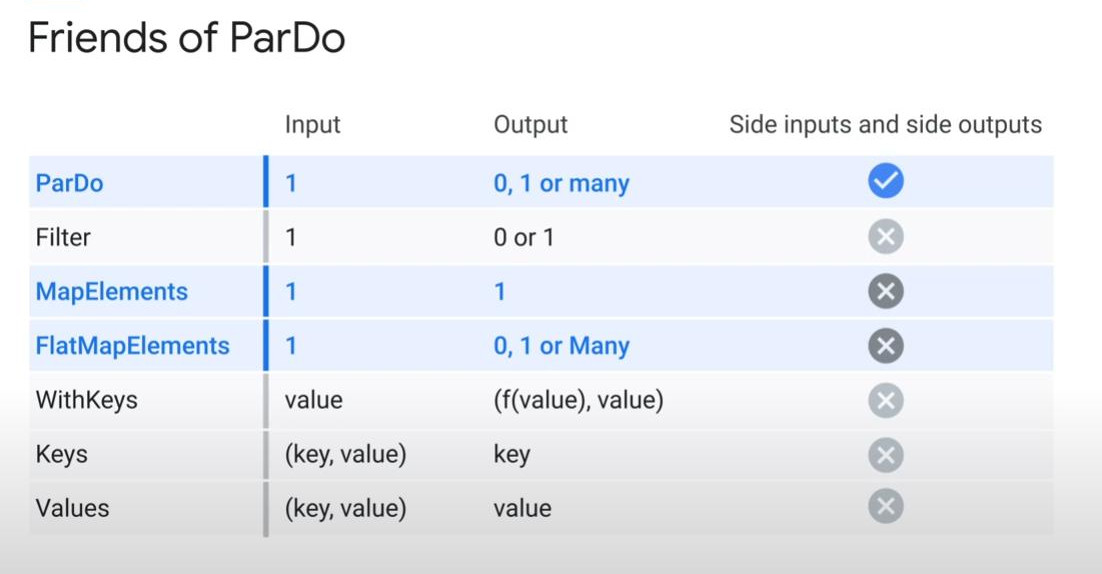
        • DoFn() Life cycle: Don’t forget that “DoFn” also offers us very powerful possibilities. Let’s see them in more details:

          • In Apache Beam, data processing operates on bundles of elements. A single bundle may contain several different keys. PCollections are automatically and arbitrarily divided into bundles, and these bundles are dynamically selected by workers. This design enables efficient parallel processing, and allows workers to retry anytime if there is a failure. For example, “streaming runners” may prefer to process and commit small bundles to reduce latency, while “batch runners” may prefer larger bundles to optimize throughput.

          

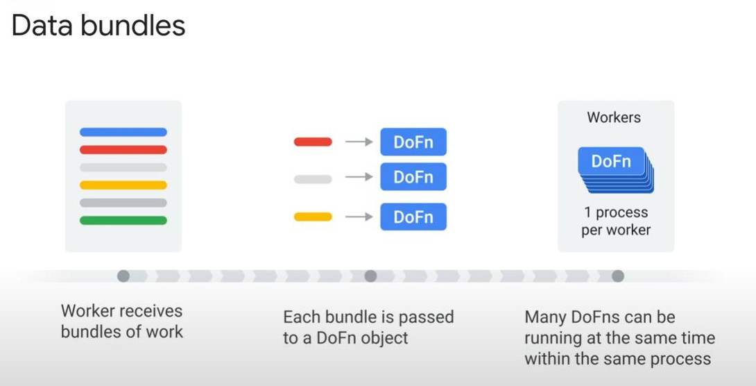
          • Method “DoFn” has several methods that can be overdriven to control how our code interacts with each data bundles. The main method is “def process” where elements are transformed. Other methods are called at different moment during the lifecycle of the method “DoFn”. These methods in combination with “side-input” and “side-output” open a myriad of possibilities for writing the “DoFn” funcion.

          

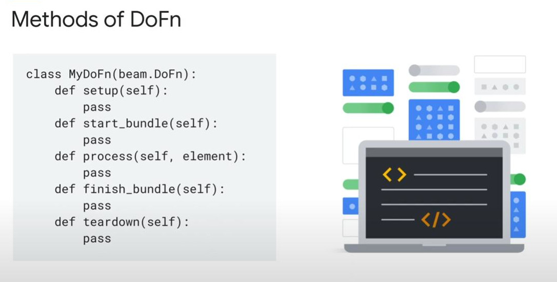
          • State variables: “State variables” are associated with individual keys in a streaming pipeline. These variables persist across multiple bundles and are updated after each processing step, ensuring correct stateful operations.

          

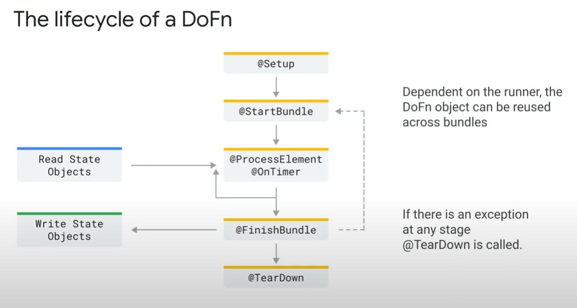
          • Beam tour in Python, and Beam college with certificate, Aggregation transforms, exercise, presentation

    • Windows, Watermarks, Triggers: Streaming with Dataflow.

      • There are 3 main concepts:

        1. How to group data in windows.
        2. The importance of watermarks to know when a window is ready to produce results.
        3. How to control WHEN and how many TIMES the window will emit output.

      • Windows

        • Processing data in batch = batch pipelines are often run on schedule, for instance, once a day.
        • The batches: are artificial split to simplify the processing of data.

        • If your data is not stationary, Beam will let us to handle it as a stream of continuous data. However, dealing with a stream is not a matter of continuity and making split to process data, there are other inherent problems to processing data as streaming such as “out of order in streams”.

        • Windowing divides data into time-based, finite chunk. A window is just a way to split data in groups to some transformation with the data.

        • Note: Some aggregations like GroupByKey and Combiners require “windowing”. But we can also do aggregation with “state and timers” without using windowing.

        • Event-time and processing-time: are 2 dimensions of time in a streaming pipeline.

          • Processing time: Dataflow assign a current timestamp to every new message.
          • Event time: the timestamp of the message set in the original source when the message was produced. This opens possibilities of doing complex and sophisticated calculations in streaming pipelines even in cases of out-of-order delivery.
        • 3 different types of window: fixed, sliding, session. (custom window is optional)
          1. Fixed window: data is divided into tiny slices (5min for each or 1 hour for each), so there is no overlapping intervals between windows.
          2. Sliding time window: map overlap, for example, a window may capture 60s source of data but a new window will start every 30s.
          3. session window: it capture bars of each activity. it is defined by minimum gap duration and triggered by another element. It’s data-dependent not time-dependent, we need to look at it to figure it out.

        

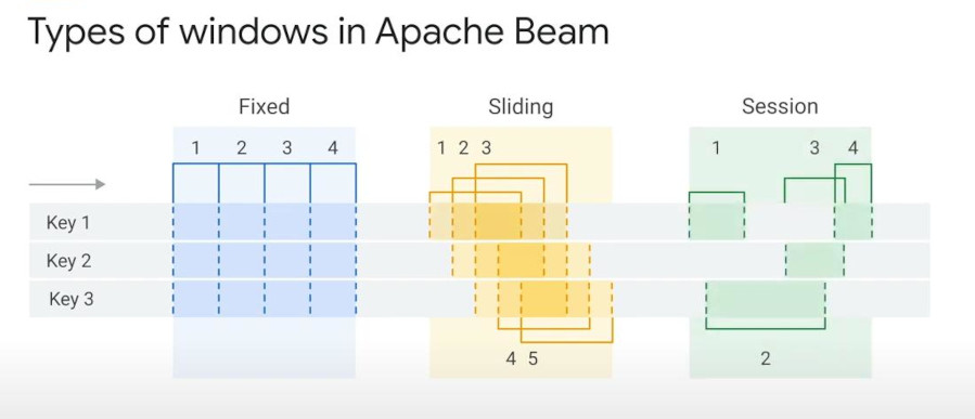
      • Watermarks:

        • What is late data? it’s very intuitive with fixed windows or sliding windows with a definition: data is late when its event-time is earlier than watermark plus allow_lateness. But if windowing is based on event-time (session windowing), it might not be obvious anymore but it’s still there with same definition: Let’s say:

          • Watermark reaches 12:00:00 event_time
          • Processing time can be anytime 11:00:00 (smaller) or 13:00:00 (larger than the watermark)
          • Set allowed_lateness = 2 minutes based on event_time
          • Beam will accept late events that have.
          • Event_time ≥ 12:00:00 → on time
          • 12:00:00 > event_time ≥ 11:58:00 → late but within allowed lateness ✅

          • Event_time < 11:58:00 → too late ❌ (event is discarded or sent to side output)

          • Note: watermark can move forward to 12:01:00 as window is still not closed
          • 12:00:00 > event_time ≥ 11:58:00 → late but within allowed lateness ✅
          • And, event_time < 11:59:00 -> too late ❌
        • How long will we wait for late data? This is where the concept of watermark becomes useful.

        • Even when we receive messages in perfect order, when they are processed in a distributed system, different messages will take different processing times and that order will be lost.

        • How can we assure that no further or other message will be received?

        • The relationship between the processing timestamp and event timestamp will define the watermark. The processing timestamp is the moment the message arrives at the pipeline. Ideally, both of the times are equal with no delays, however this rarely happens. There are always latencies and so on. Watermark is an added extra time which Dataflow will use to wait and define whether a message is later or not. Any messages that arrive later than “watermark” is set “later”.

        

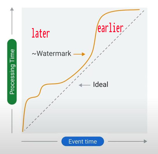
        • Watermark helps to decide when a window is complete. In other words, Dataflow will wait until the watermark is trespass to close the window. We need to decide how to do with these later messages, by default they are dropped.

        • Data freshness - (Latency) is the difference between the current real-world time and the event timestamp of the latest message waiting to be processed. The “watermark” is actually the event timestamp of the oldest message that has not been processed yet. So, watermark is a point of event_time and always changing and moving foreward.

        • System Lag - (Sys Latency): a period of time the system takes to fully process a message. If in some cases the system need more time process a message, the system lag (latency) will increase.

        • If latency increases monotonically but the sys latency keeps unchanged. That means, there are more messages arriving at the pipeline, but the system still can process at the same space, so latency does not increase the system latency. At this time, Auto-scaling will add workers to process the waiting messages.

        

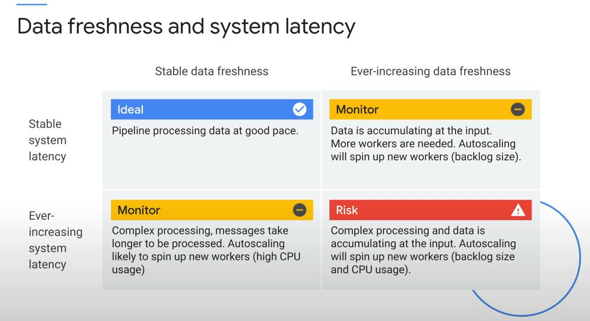
      • Triggers: used to check some results of processing early or whether late data is under control with custom triggers like following: (we cannot let the processing running alone, we have to check results at runtime so we need triggers)

        • Triggers can work on event-time, processing time, data-driven, or a composition of them. By default, we have a afterwatermark trigger that is an event-time trigger.

        • Note: triggers also help to check late data for our additional process.

        

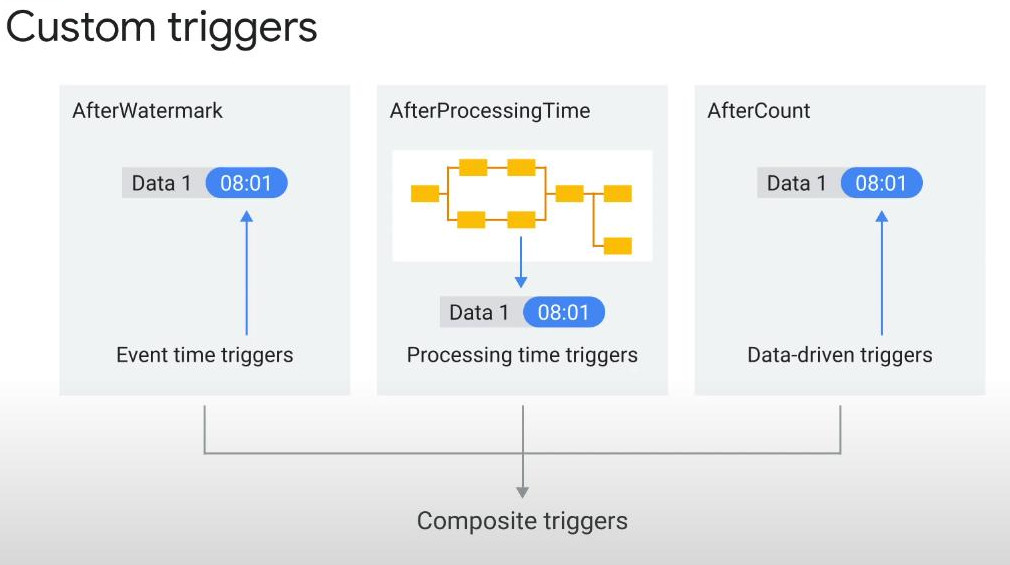
        • Accumulation mode: if we trigger a window several times, (how apache-beam repeats calculation), we need specify the desired accumulation mode. There are 2 types of mode:

          • ACCUMULATE mode: apache-beam will repeat calculation with all the data included in a window regardless of number of triggers we made to the window.
          • DISCARD mode: the calculation only include the new data (since the latest trigger) that has never been included in any calculation to previous triggers.

          

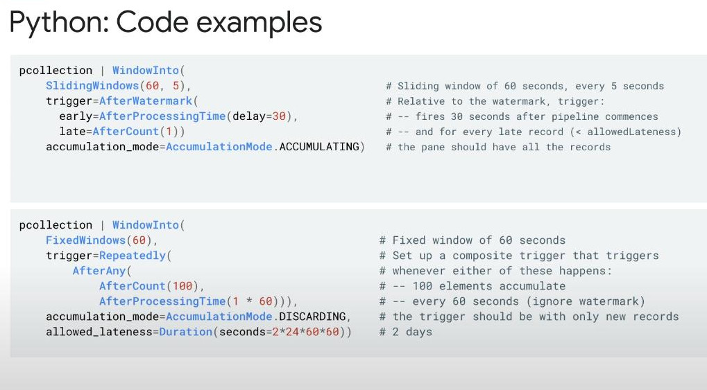
    • Sources(E) and Sinks(L) (in th ETL pattern): Mr.Wei Hsia - Customer Engineer: Below are common sources or sinks we can meet on Cloud:

      1. Sources and Sinks (in Beam) they are basically an input and an output in a Dataflow pipeline. A source appears at the beginning and a sink is a PTransform that performs a write to the specified destination. Sink will emit a PDone value to signify the completion of the transform.

         • A bounded source == a chunk == a bundle = a unit of work (bundles can even split into smaller chunks for better performance by runners.)
           • Because these bounded sources are finite, Dataflow can provide an estimate of number of bytes to be processed, even a start point end an end point of a process.
         • An unbounded source is associated with streaming.
           • Checkpoints: to bookmark where data has been read to avoid reading the same data.
           • Watermark: is a point of time to define when a window is complete.

      2. TextIO & FileIO:

         • TextIO: both read and write

           • For a single file: ReadFromText(file_name)

           • For a list of files:

                 "create" >> Create([file1, file2])
                 "read" >> ReadAllFromText()
             
                 "write" >> WriteToText(known_args.output, coder=JsonCoder())
             

         • FileIO:

           • Use a file pattern or regex to filter matched files:

             with beam.Pipeline() as p:
                 readable_files = (
                     p
                     | fileio.MatchFiles('hdfs://path/to/*.txt')
                     | fileio.ReadMatches()
                     | beam.Reshuffle()
                 )
             
                 contents = (
                     readable_files
                     | beam.Map(lambda x: (x.metadata.path, x.read_utf8()))
                 )
             

           • FileIO is even able to monitor continuously a location for a pattern. For example, it can check new coming data in a location every 30s for an hour.

           

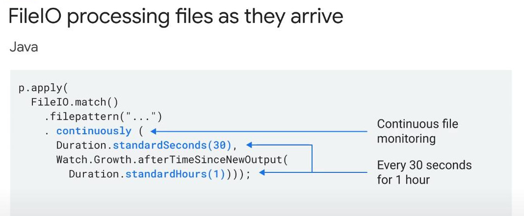
           • FileIO can process files as they arrive. Below methods is used to read a stream of files (streaming data)

             with beam.Pipeline() as p:
                 context = (
                     p
                     | beam.io.ReadFromPubSub(...)
                     | ReadAllFromText()
                 )
             

           • We also have ContextualTextIO.read() for advanced usage like dealing with windowed writes, with file-based triggers, side inputs, stateful file writes, or context-aware destinations. ()

           • We can even set a dynamic sink with FileIO:

               p
               | beam.io.fileio.WriteToFiles(
                  path='x/y',
             
                  desination=lambda record: 'avro' if record['type']=='A' else 'csv',
             
                  sink=lambda dest: AvroSink() if dest=='avro' else CsvSink(),
             
                  file_naming=beam.io.fileio.destination_prefix_naming()
             )
             
             

      3. BigQueryIO: is a useful connector for Bigquery.

         • BigQuery Storage API supports Dataflow pipelines with parallel-reading on BigQuery but only Java SDK supports it. Python SDK does not natively support but it has a package “bigquery_storage” to support it we can use it separately like fetching first, then put results into pipeline later like below.

             from google.cloud import bigquery_storage
             import apache_beam as beam
         
             def fetch_data():
                 ## use BigQuery Storage API here
                 return list_of_rows  ## Convert to a format Beam can process
         
             (p | beam.Create(fetch_data()) | <further processing>)
         
         

         • Without Storage API, we can read tables directly with beam.io.ReadFromBigQuery() like below:

             (p
             | 'QueryTableStdSQL' >> beam.io.ReadFromBigQuery(
                 query='SELECT max_temperature FROM' \
                 '`clouddataflow-readonly.samples.weather_stations`',
                 use_standard_sql=True)
             | 'Reading' >> beam.Map(lambda elem: elem['max_temperature']))
         

         • BigQueryIO also supports writing with dynamic destinations (multi-destination) even with various schemas as well. We can define a separate function to dynamically return the destination we would like data routed to like following image:

         

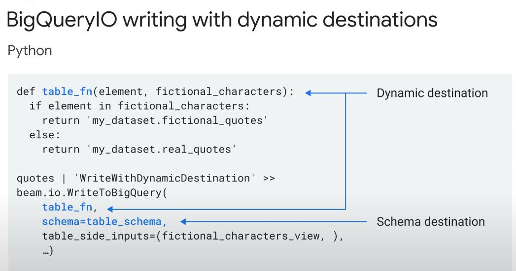
      4. PubsubIO: Dataflow and Pubsub can go hand in hand, they can connect via PubsubIO.

         • PubsubIO has ability to pass a record ID that helps de-duplication in pipelines by comparing IDs.

         • Reading: While reading, PubsubIO auto creates a subscription when Dataflow job is deployed and destroys the subscription upon the termination of the job. But we can keep the subscription if necessary like below:

         beam.io.ReadFromPubSub(topic=ABC)  --auto delete as job terminated
         
         beam.io.ReadFromPubSub(subscription='project/')  --subscription remains
         beam.io.ReadFromPubSub.fromSubscription('project/')  --subscription remains
         

         • Capture failure == PubsubIO write if a message was 5 times failed while sending, we could capture and put them in a bucket. The configuration is below, first we define subscription with –max-delivery-attempts=5 and then use “PubsubIO” to write failed messages to the dead-letter-topic bucket

         gcloud pubsub subscriptions create my-subscription \
         --topic=my-topic \
         --dead-letter-topic=projects/YOUR_PROJECT/topics/my-dead-letter-topic \
         --max-delivery-attempts=5
         
         
         messages = (
             p | "ReadFromPubSub" >> beam.io.ReadFromPubSub(
              subscription="projects/YOUR_PROJECT/subscriptions/my-subscription")
         )
         
         processed = (
             messages | "ProcessMessages" >> beam.ParDo(process_message)
             .with_outputs("failed", main="main")
         )
         
         processed.failed | "WriteFailedMessages" >> beam.io.WriteToPubSub(
          "projects/YOUR_PROJECT/topics/my-dead-letter-topic")
         
         

      5. KafkaIO:: is an unbounded source used for streaming. KafkaIO is built in Java but beam still has come cross-language transform like ReadFromKafka in Python.

      6. BigTableIO:: BigTable is a NoSQL database service by Google. Both BigTable and Dataflow are highly scalable and they communicate by BigTableIO (read and write).

         • Row Filter: able to do a RowFilter using row key.
         • Prefix Scan: like any NoSQL database, it is able to do prefix scan using row-key as index.
         • Wait.on(): force the pipeline runner to wait for the writing to complete before other transforms, (only in Java). Python SDK handles this waiting automatically.

      7. AvroIO: “.avro” is a file-format that is popular for big data. AvroIO enable us to read/write this file type. In Java, all “avro files” are self-describing with schema files under “avsc” format (schema_file.avsc). Nod need for Python

         (
         pipeline
         | 'ReadFromAvro' >> ReadFromAvro(input_avro_path)  #This reads the Avro files
         | 'ProcessAvroData' >> beam.Map(process_avro_record)
         | 'WriteToJson' >> beam.io.WriteToText(output_path))
         
         

      8. Splittable DoFn: brings Beam closer to fruition (golden time). The core key is splittability of a big job which we cannot process in parallel like reading a big file. It allows to build custom sources (reading) with ease as below:

         • def initial_restriction, shown in following image, will create a restriction defining a complete unit of work.
         • a tracker then is created to monitor this new restriction by def OffsetRestrictionTracker
         • Details in here

    • Schemas: a way to express data structures in pipelines.

      • byte string : only 256 ASCII characters in the form of digit 0-255

        string or plain text : all kinds of human-readable characters in format of unicode. String can be encoded to byte string with my_byte_str.encode(“utf-8”).

      • UTF-8 is not a character set, it’s an encoding, it tells how to store Unicode characters using 1 to 4 bytes, including over 1 millon encodings (characters) from Greek, math, chinese, vietnamese, symbols,…
        • Pipeline records: one record in one element in PCollections.
        • Why we need schemas in beam pipeline:
          • Naming a new fields as appearing.
          • Type safety.
          • As writing into a sink like BigQuery or BigTable.
        • PCollection must have a schema attached to it. One PCollection only has one schema.

    • State and Timers (fine-grained control): a powerfull tool we can use in a DoFn to implement stateful transformations:

      • State API: Pardo is normally a stateless transform that cannot aggregate elements like GroupByKey or CombinePerKey. Pardo can only do mapping, map element to a function and yield a list. But is it changeable? Apache Beam adds this stateful feature to Pardo, which is then called stateful Pardo, by reusing stateful variables. This means Pardo can do aggregations.

      • Why aggregations refers to state? it’s because state is a memory of streaming, and total number (or aggregation) needs to be saved and updated continuously in memory while streaming. So, aggregation represents a state of streaming.

      • In a pipeline, state is also maintained per window and local to each transform. In other words, two different keys processed in 2 different workers are not able to share a common state but elements in the same key can share a common state.

      • We can see 2 state variables in the following example. ParDo only stop entirely when the whole state are clear. (the purpose of this state here is that we do batch-by-batch calls (after num-elements reachs a MAX) instead of element-by-element calls to avoid overwhelming external services, that is omitted for simplicity)

      

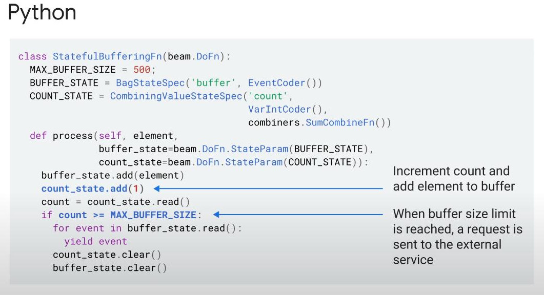
      • What if the state does not reach the MAX after the final message? => refer to the Timers

      • Timers API: combines with State API to have more perfect stateful transformations.

        • Ensure a state is cleared at regular intervals of time. As with the case of windows and triggers, we can define TIMERS either in event-time or processing-time.

        • Event-time timers: depends on the watermark value, for instance, invoke a callback when the watermark reaches some threshold. Event-time timers are influenced by the rate of the progress of input data.

        • Processing-time timers: depends on the clock of worker, not on any kinds of timestamp included on a message, invoke a callback after a certain amount of time has elapsed. Processing-time timer will expires regardless of the progress of the input data. The timers will clear at regular intervals.

        • If a ParDo is processing the last message of the last bundle, it’s likely that the buffer will not reach the threshold set in the code or the message might be coming very slowly, in both cases we also want to produce results rather than waiting very a long time for the message to show up. Timer will help with this.

        • An example of event-time timer in the following example:

        

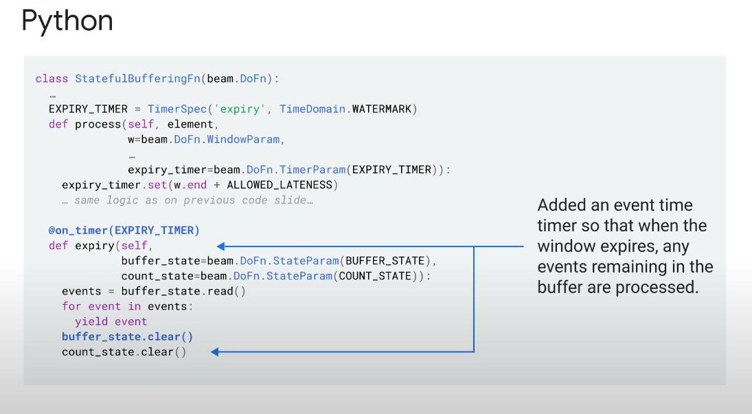
      • Types of state: state_examples

        1. Value: single value
        2. Bag: a list of values
        3. Combining: a kind of aggregation like “sum”, “count”
        4. Map: a pair of key + value
        5. Set: only unique items

    • Best Practices:

      1. Beam Schemas:

         • Make our pipeline code more readable and cleaner
         • Allow Dataflow service to make optimization behind the scene as it is aware of type and structure of data being processed. For ex, Dataflow service optimizes data serialization and deserialization using encoders and decoders as the data flows through different stages in a pipeline, serialization and deserialization become faster with available schemas without additional steps of prediction.

      2. Handling erroneous data & Error handling:

         • rather than just log erroneous records, sending the log data to a persistent storage medium such as BigQuery or Cloud Storage to handle separately.
         • In the process method of ParDo function, considering using try/catch block. In the try/catch block, avoid logging every error exception as it may overwhelm the whole pipeline especially when “presenting errors” increases, instead, sending all erroneous records to an alternative sink for further inspection. These records should be tagged “DeadLetter”. For success records, it is written in different sink.

      3. AutoValue code generator: is a utility class that Beam SDK provides for generating POJOs which stands for Plain or Java Objects.

         • Although Beam schemas are the best way to represent objects in a pipeline due to their intuitive structure, there are places where a POJO is needed, such as handling key-value objects or stateful objects.

         • Use AutoValue class builder to generate POJOs when not using schemas. AutoValue is used popularly in Beam code-base using Java SDK. For Python, NamedTuple is used instead.

      4. Json data handling:

         • handling Json strings in Dataflow is a common need. For Java, use a built-in method JsonToRow. For Python SDK, use json.load(e).

         • In case we need to convert from Json to POJOs, use the AutoValue class with the “@DefaultValue” annotation.

         • Struture of json data may change frequently, use DeadLetter Pattern to handle unsuccessful messages or exceptions.

      5. Utilize DoFn lifecycle:

         • What is the “life cycle of DoFn objects” for micro batching?

         

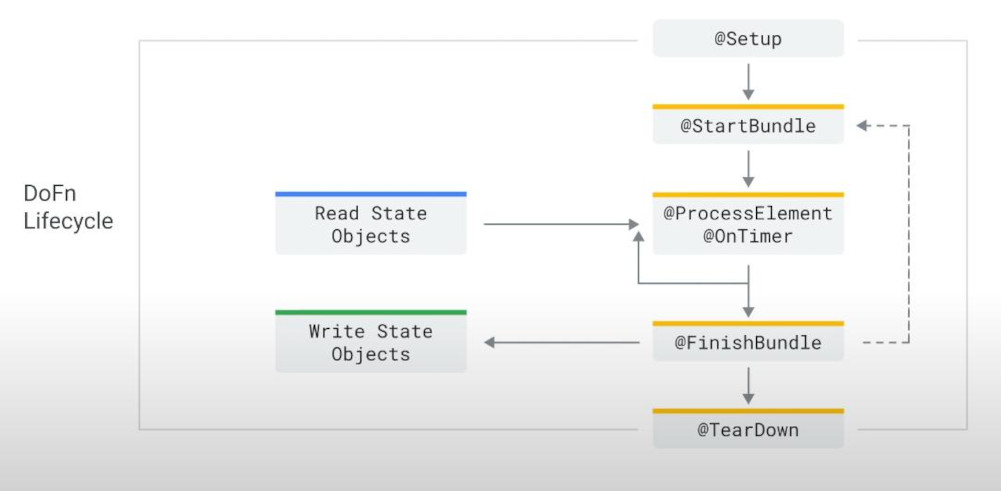
         • Issue: in a big data use case, it is easy to overwhelm an external service endpoint (API) if we make a single call for each input element without applying any reducing function.

         • Solution: If remember, we recommended “batching calls” to an external API by leveraging two life cycle methods “StartBundle” and “FinishBundle”. For mirco batching, we can initialize or reset the batch in the “StartBundle” and commit it in the “FinishBundle”, please note that due to “Dataflow runner operation” these two methods can be called multiple times to process more than one bundle. Because data is split into bundles by Dataflow runner. Each bundle is a batch of elements processed together in parallel. A single DoFn instance might process multiple bundles over time. Hence, for each bundle, “StartBundle” and “FinishBundle” will be called one time.

         

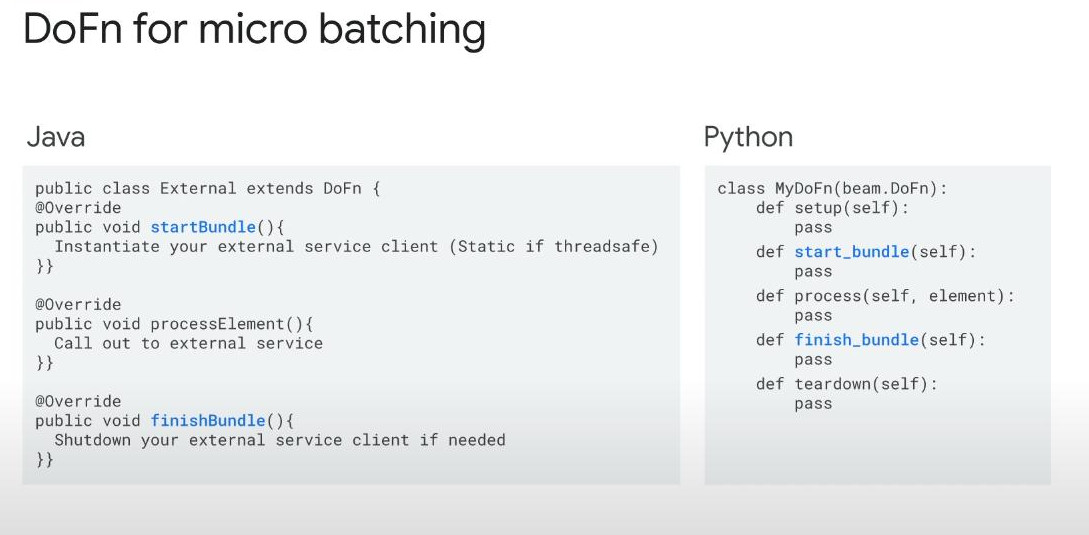
      6. Pipeline optimizations: some general guidelines we should keep in mind while developing our pipelines:

         • Filter data early whenever possible: This will reduce data volumne flowing through the pipeline, thereby enabling efficient use of the pipeline resources.

         • Data collected from external sources often need cleaning.

         • Whenever possible, apply data transformations serially to let the dataflow service to optimise DAG for us. “Transformations applied serially” is suitable for “graph optimization” because multiple steps can be fused together behind the scenes in a single stage for execution on the same worker, thereby reducing costly IO and network operations. (By executing these fused steps on the same worker, Dataflow reduces the amount of data transferred over the network.)

         • Handle back pressure from external systems. For instance, if writing into an external system like BigTable can have high write latency, resulting in an bottleneck issue. So, it is recommended that we should manage the APPROPRIATE capacity of the external system to avoid back pressure.

         • Enable “autoscaling” is also a good idea to reduce number of under-utilized workers.

    • SQL and DataFrames(having a similar interface of Pandas).

      • Dataflow SQL: helps using SQL in a data streaming code:

        • Use cases: Select from PubSub, Join with batch data, Aggregate over Window, Publish to BigQuery of PubSub.
        • It’s planned to integrate with other Google services like Kafka or Bigtable.

        • Note that: with Dataflow SQL we use Dataflow engine to execute SQL statements instead of our common BigQuery engine. It’s important to ensure the regional endpoint, sources, and destination are within the same region if possible.

        • Besides SQL in-pipeline, we can use SQL in command line - CLI (shell) with Dataflow SQL CLI.

        

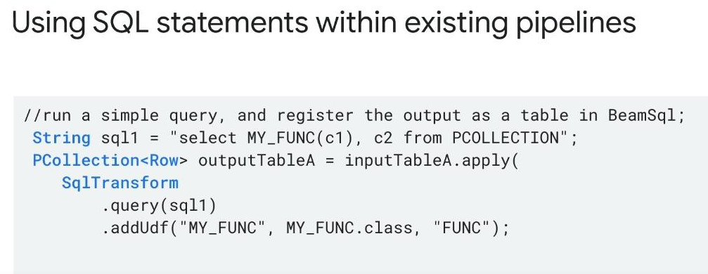
      • Beam SQL : can be embedded in an existing pipeline using SqlTransform, which can be mixed with PTransforms. In Java, it also supports some UDFs (user-defined functions)

      • Suport multi-dialects: two main types.

        • Calcite SQL : The SQL (via Apache Calcite) used by Beam SQL to parse and execute SQL queries over data streams. It also lets us write SQL queries against PCollections in a declarative way to process data without writing Java/Python code.

        • ZetaSQL : developed by Google in products like: BigQuery, Cloud Spanner, Google Sheets (query parts), Looker, Dataflow SQL.

      • Windowing in SQL:

        • For Fixed Window:
          • TUMBLE() defines non-overlapping fixed windows of 1 minute.
          • TUMBLE_START() gives you the start time of each window.

        SELECT
            TUMBLE_START(event_timestamp, INTERVAL 1 MINUTE) AS window_start,
            COUNT(*) AS event_count
        FROM pubsub.topic.`your-project.your-topic`
        GROUP BY TUMBLE(event_timestamp, INTERVAL 1 MINUTE)
        

        • For Sliding Window:
          • HOP(event_timestamp, slide, window_size) creates sliding windows.
          • INTERVAL 5 MINUTE → the hop/sliding interval (how often a new window starts).
          • INTERVAL 10 MINUTE → the window size (how long each window lasts).

        SELECT
            user_id,
            HOP_START(event_timestamp, INTERVAL 5 MINUTE, INTERVAL 10 MINUTE) AS window_start,
            HOP_END(event_timestamp, INTERVAL 5 MINUTE, INTERVAL 10 MINUTE) AS window_end,
            COUNT(*) AS click_count
        FROM click_events
        GROUP BY user_id, HOP(event_timestamp, INTERVAL 5 MINUTE, INTERVAL 10 MINUTE)
        

        • For Session Windows:
          • SESSION(event_time, INTERVAL 15 MINUTE) groups events that are less than 15 minutes apart into the same session.
          • SESSION_START and SESSION_END return the actual session window boundaries.

        SELECT
            user_id,
            SESSION_START(event_time, INTERVAL 15 MINUTE) AS session_start,
            SESSION_END(event_time, INTERVAL 15 MINUTE) AS session_end,
            COUNT(*) AS page_views
        FROM clickstream
        GROUP BY
            user_id,
            SESSION(event_time, INTERVAL 15 MINUTE);
        
        

      • Beam DataFrames: a more Pythonic Cloud API (compatible with Pandas DataFrames)

        • Parallel processing with Beam model could be slower than Pandas DataFrames.
        • Beam DataFrames and Beam SQL is a type of DSL in Beam Python SDK.
        • NOTE: Beam DataFrames can be used to replace beam transform like ParDo or CombinePerKey.

        • Easy programming interface within Beam pipeline and somehow more efficient with vectorized pandas implementation.

        • LIMITS of Beam DataFrames:

          • Cannot transpose like ordinary Pandas

          • Results of most operations are not available till the end of a pipeline. For instance, we can compute a sum() but cann’t branch it with IF sum() > 100 ELSE … because result of sum() is only available after finishing a pipeline. The only thing we can work is the columns NAMEs and TYPEs from the beam schema, not the results.

          • PCollections are not in order, so any Pandas operations sensitive to the ordering will not be supported like head, tail, or shift.
        • Example of Counting Words with Beam DataFrames:

        

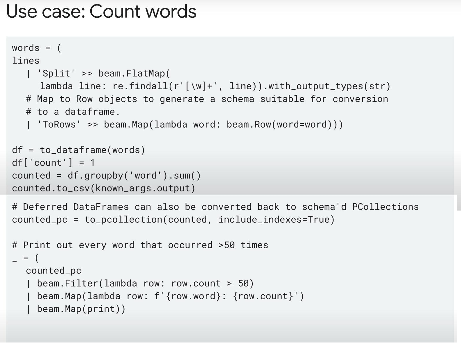
    • Beam Notebooks.

      • Similar to Colab that is limited to the local environment. It’s not serverless or scalable, only useful for experimentation.

      • Example of dataflow fusion:

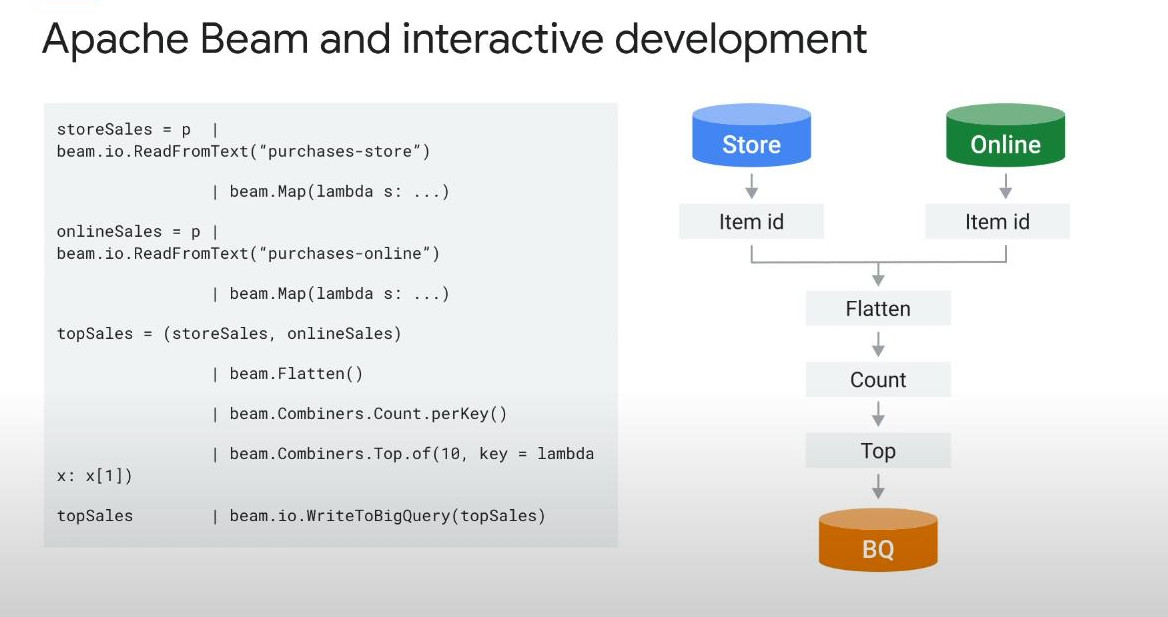
      • What an interactive runner can allow us to do with .head(n) or .visualize():

        • Get access to intermediate results (PCollections after each transform)
        • Able to work with both batch and stream sources.

      • How we tell the runner when to stop recording/reading: 2 options

        • ib.options.recording_duration : set a fixed amount of time

        • ib.options.recording_size_limit : a fixed amount of bytes, which is very useful for a real case of streaming when you may have a very large volumne of data.

        • Some other useful methods:

        • ib.show(windowed_word_counts, include_window_info=True) : materializes the resulting PCollection into a table.
        • ib.collect(windowed_word_counts, include_window_info=True) : load the output into a Pandas DataFrame which we can do some manipulation against (Pandas table).
        • ib.show(windowed_word_counts, include_window_info=True, visualize_data=True) : visualize the data in the notebook.

        

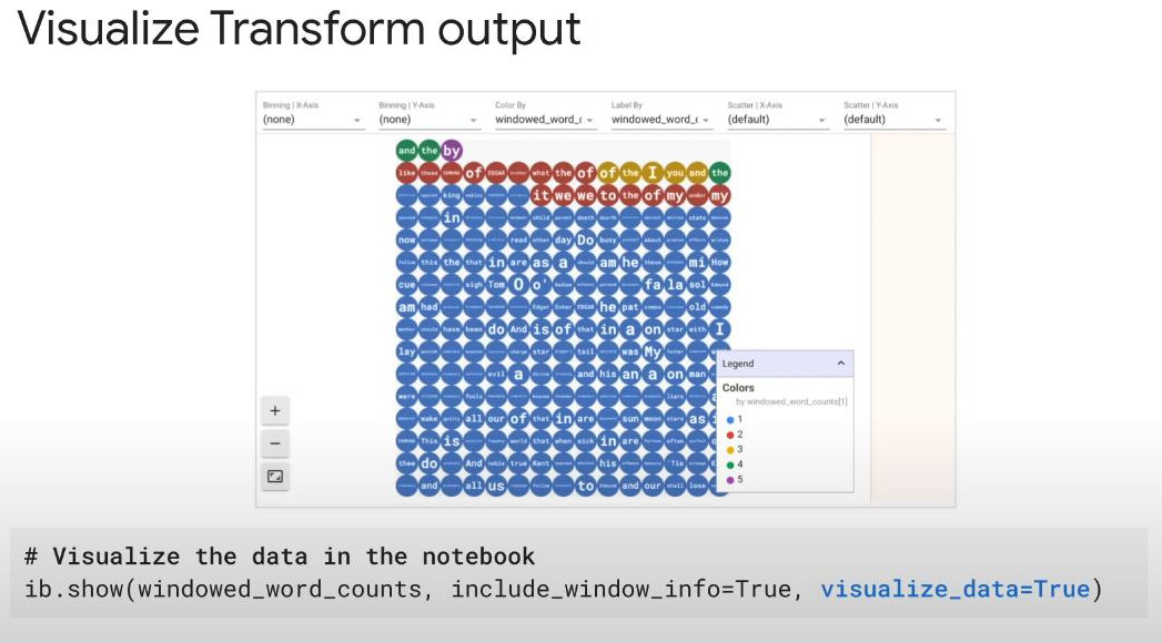
      • Re-use feature: is an important option that we can choose to actually reuse the stream of information that we have gathered OR to get fresh data. This first is useful to prevent repeated reading the same dataset, saving cost of reading. The latter is useful to give us the most updated information because stale data could lead to wrong decisions.

      • Code to submit our code to the production:

          from apache_beam.runners import DataflowRunner
          options = pipeline_options.PipelineOptions()
          runner = DataflowRunner()
          runner.run_pipeline(p, options=options)
      

25. Dataflow Operation:

    • Monitoring:

      • Job list : Cloud Monitoring is integrated tightly with Dataflow. The fist page of Dataflow will show a list of jobs, we can do some filters, sorting, and bookmark the view with specific filter and sorting if necessary.

      • Job Info : After clicking one job, we will see the job info. On top right is the metadata (encryption type), below is resources in use (CPUs, Memory), next is the parameters used to run the pipeline.

      • Job Graph = DAG : a visually representation for each step, which might be made up of sub-steps.

        • For Batch data: steps are executed sequentially, the next part should not start until the one before it finishes. Dataflow optimizes all steps by split them into various optimized stages that can be shared among pipeline steps. Jobs do get completed with batch pipeline.

        • For Streaming data: all the steps will run concurrently. There is no completion time for jobs unless we cancel or drain it.

        • Throughput: total amount of elements per second.

        • Wall time: total amounf of time by the assigned workers to run each step. It’s useful to check which step our workers take longer time to run on.

        • Note: Some custom metrics we might need to track a specific data feature. We can also see them at the right pane of the Dataflow Job Graph Page.
          • Counter: increment and decrement
          • Distribution: COUNT, MIN, MAX, MEAN
          • Gauge: latest value

        

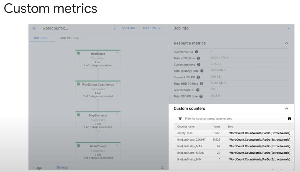
      • Batch Job Metrics Tab or Page:

        • The first graph: track the number of workers

          • Dataflow decides more or less workers are needed to maintain the perfect job throughput.
          • The green lines shows the number of workers needed, the blue line shows the current number of workers running.

        • The second graph: show the throughput of each sub-step versus time.

        • The third graph: for CPU utilization

          • A healthy pipeline should have all the workers running at around the same CPU utilization rate.
          • Uneven distribution workload: means few workers work 100% while others do nothing because of heavily skewed data.

        • The final graph: “Worker error log count”:

          • Shows the number of log entries from workers that had a level of error.

        • Notice: in batch pipeline, if processing an element fails four times in a row, the whole batch pipeline fails.

      • Streaming Job Metrics Page: similar to the batch job metrics with some following extra metrics:

        • “Data freshness” and “System latency”: very useful to measure the health of a streaming pipeline.

          • Data freshness: shows the difference between “real-time” and the “output watermark”.

          • The watermark is a timestamp where any element timestamp prior to it is nearly garanteed to have been processed. For example, if the current timestamp is 9:26am and the data freshness graph shows 6 minutes at that time. This means all elements with the timestamp at 9:20am or earlier have arrived and have been processed.

          • When data is seen to be “fresh”? data is “fresh” when it is processed almost in real time without a big lag.

        • “System latency”: shows how long it take elements to go through the pipeline.

          • If the pipeline is blocked at any stages, the latency will increase. For example, we have a pipeline reading from a PubSub, do some transformation, then sink into a Spanner. Suddenly, the Spanner goes down for 5 minutes. When this happens, PubSub won’t receive confirmation from Dataflow that element have been sunk into Spanner. This confirmation is needed for PubSub to delete the element, so the system latency and data freshness both will rise 5 minutes. When Spanner returns to work, Dataflow sends confirmation to PubSub, returning the system latency and data freshness to normal.

        • “Input metrics” or “Output metrics”: they will show up when our pipeline reads and writes records using PubSub respectively.

          • If I have over 2 PubSub sources or sinks, we can select one of them to see its metrics as following:

          • “Request per sec” : it is the rate of API request to read or write by the source or sink over time.

            • If the “Request per sec” drops to 0 or decrease significantly, our pipeline should be blocked at certain steps. When this happens, we should review first the steps that have high watermark to check the blockage. Additionally, we can check the “Worker error log count” to see errors or indications.

          • “Response errors per sec by error type”: it is the rate of failed API requests to read or write by the source and sink over time. If an error happens, take the code and cross-reference it to the specific error code in the documentation.

      • Custom Dashboard:

        • Cloud Monitor is integrated tightly with Dataflow to track time-series data to provide viewing and alertings:

        • Custom dashboard means we can show on our dashboard any metrics that we are interested at. Below is some common metrics we should consider.

        

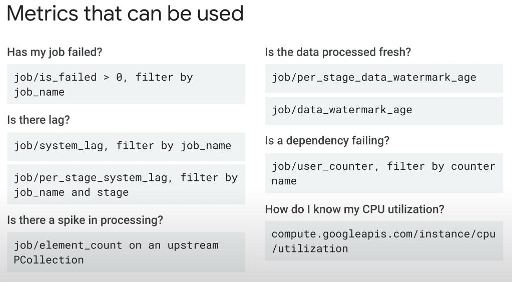
        • Most of metrics that we have seen had a “Create alert policy” button. This allows us to set alert and be noticed when a certain metric crosses a specific threshold. This becomes useful when in streaming pipeline, if an element fails to get processed, it is retried in-definitely (forever) unless we cancel or drain a job. We can catch the number of retries by setting an alert if system latency increases over a predefined value. Every time an alert is triggered, an incident and a corresponding event are created, if we set the notification mechanism in the alert such as an email or SMS, we will receive the notification.

        • Note: The alert policy provided is on per pipeline but we can build a custom alert policy grouping over one pipeline using Cloud Monitoring.

    • Logging panel (in job graphs) and centralized Error Reporting:

      • The logging panel is located at the right bottom of the Dataflow job graph page. There are 3 tabs: job logs, worker logs, and diagnostics

        • Job logs : logs or errors from Dataflow services
        • Worker logs : messages are from VMs that managed all the workers running the job.

        • Diagnostics : a link to Error Reporting page, the first seen, the last seen. Additionaly, Diagnostics tab also shows “jobs insights”:

          • If submitted file into workers missed some required classes, we will receive an error message of “Worker jar file misconfiguration”

          • If our coding took a long time to perform operations, we might see a operation link in the diagnostics tab. If the slow processing due to “Hot key detected”, the diagnostics tab will show the message “Hot key detected”. (“Hot key” means some key has a large scale over others as performing GroupByKey or CombinePerKey)

          • In streaming scenario, our pipeline will fail to process if we are grouping a huge amount of data without using a combine transform or producing a large amount of data from a single input element. If this happens, the diagnostics will notice “Commit Key request Exceeds Size limit”. To avoid this, we should do pre-aggregations before heavy operations like windowing or grouping. But before pre-aggregation, we need to set key if data structure is not a key-value type. There are 2 ways to declare key: beam.Map(lambda x: (k, v)) or beam.GroupBy(‘key’).aggregate_field(‘user_id’, sum, ‘page_views’). Now, CombinePerKey() will combining data locally on each workers before shuffling results out for further combining. This will reduce the amount of data significantly compared to method GroupByKey().

          • Finally, if there are a high rate of logging msgs, some of them could not be sent to your Cloud Logging, “Throttling logger worker” warning will appear in our Diagnostics tab.

          • We should see another log tab for BigQuery if our pipeline reads/writes data to BigQuery. (required BigQuery Admin and beam 2.24+).

            • For reading BigQuery: both extract jobs and query jobs are shown in the Diagnostics tab. (the first: BigQuery will send all the table under JSON format to GCS using “extract jobs”, the latter: BigQuery sends a part of a table under JSON format to GCS using “query jobs”)

            • For inserting data to BigQuery: only load jobs are shown. “streaming inserts” is not shown. By default, “load jobs” are used to sync bounded PCollections and “streaming inserts” for unbounded PCollections.

            • In BigQuery Jobs tab, select the region of the dataset. click on Load BigQuert jobs to get a list of all jobs that BigQuery ran from our pipeline . We can press “Command Line” if we want to see more detailed information about the job. A pop-up window will show the gcloud command, then pressing “run in Cloud shell” button to examine the results like “destination uri”, “number of bytes”, “length of time the job took to run”. It will take any real effect to the data.

            

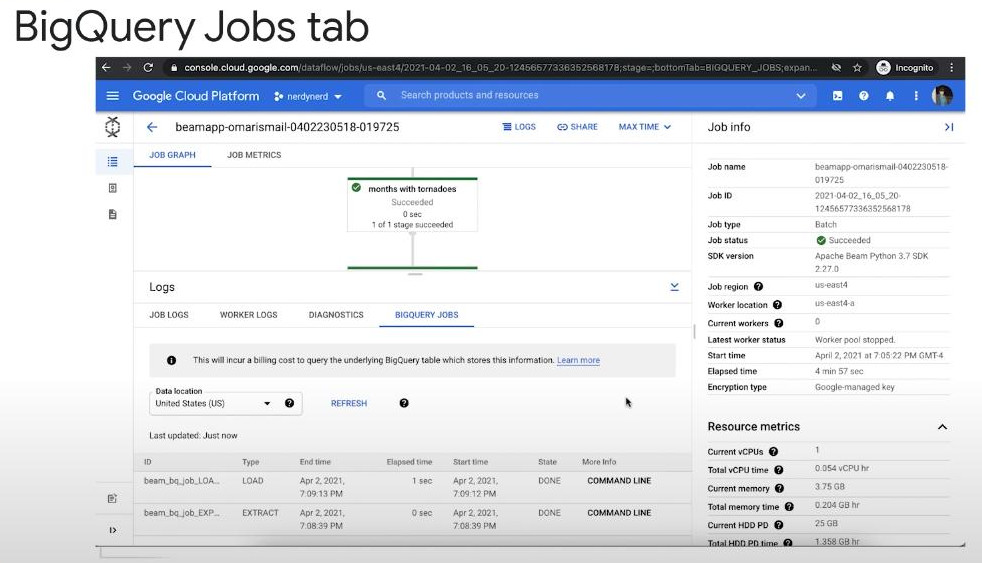
          • Error Reporting page: aggregates and displays a list of frequently occuring errors from our Dataflow pipelines in our project.

            • We can see how many times the error occured across a specific time range such as 1 hour, 1 day, 7 days…

    • Troubleshooting and Debugging: includes 2 steps

      • step1: checking for errors in the job.

        • There’s a error notification icon located above the job graph. Expanding the log pannel to show more details.
        • Cloud Logging offers a simple UI (logs panel) to filter and search for logs within the job.

      • step2: looking for anomalies in the Job Metrics tab.

        • Data freshness and System Latency are good indicators of performance.
        • Increasing Data freshness shows that the pipeline workers are unable to keep up with the rate of the data being ingested into the pipeline.

        • Increasing System Latency indicates that certain work element within the pipeline is taking a long time to get processed.

        • CPU utilization is also a good indicator for parallelism in a job and also indicate if a job is CPU-bound (100%). The below image is a good example of bad parallelism, only one or few of workers have high CPU utilizations while others close to zero.

        

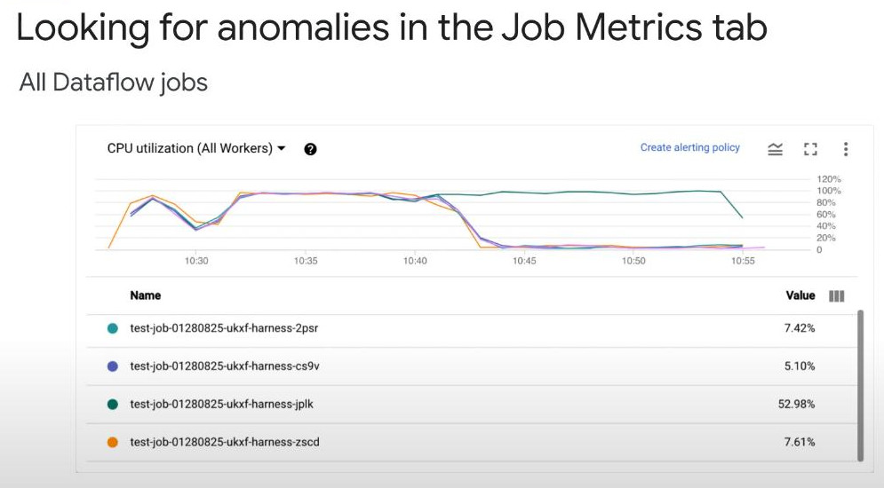
      • Types of troubles: 4 types

        • 1. Errors as building the job graph or the pipeline.
          • Validating Beam Model aspects, including input, output specifications…
          • There is no job created on the Dataflow service if there is an error as building the pipeline.

          • Common errors: GroupByKey is applied to un-bounded PCollections. (Windowing will help create bounded PCollections).

          • Notice: these errors can be re-produced by local DirectRunner.
        • 1. Errors as creating jobs.

          • After building the pipeline or the DAG graph successfully, Dataflow service then will check the following certicates:

            • Access permission to the job’s associated Cloud Storage buckets.
            • Validate permission roles to execute the project.
            • Access permission to the input and outpur sources.

          • If we want to see log messages or errors in the console or terminal window, we have to use “blocking-execution” with the “.wait_until_finish()” method. Otherwise, we can only see them in the Log panel on the botton of Dataflow graph page.

          • Notice: these errors can not be re-produced by local DirectRunner. To avoid undue costs while testing, just execute the pipeline with a tiny amount of data because these errors are not dependent on the data scale.

        • 1. Exceptions during pipeline execution.

          • These exceptions happens in the beam.DoFn method in the pipeline and are not handled properly by our code. So, they are reported as failed tasks in the Dataflow Monitoring interface (Log pannel).

          • It’s important to notice that batch and streaming pipeline handle exceptions:

            • In batch: the dataflow service will retry a failed job up to 4 times and then go for the next elements. (fault-tolerance).
            • In streaming: the dataflow service will do the same with 4 retries before passing to next elements. (fault-tolerance).
        • 1. Slow performance.: the useful UI interface to debug the performance is the Step Level with Step-Info UI. Step Info provides step title, Wall time, Input elements, Input bytes…
             • Wall time: approximate time spent across all threads in all workers in the following actions: initializing the step, processing elements, shuffling elements, ending the step.
             • Estimated size: the total volumne of data that the step has received.

    • Performance Influencing Factors:

      • Pipeline Design:

        • We should place transformations that reduce the volumne of data as high up on the graph as possible. This placement should be above the windowing.

        • If our pipeline has large windows(1hour) aggregating large volumne of data, we can create “smaller windowing(1min) + combine” patterns before the “main windowing(1hour)” to reduce the volumne of data processed on the main windows.

        • Dataflow auto optimization: is called Fusion, where adjacient transforms like ParDo will be fused together into a single stage that can be handle by one worker to generally increase performance. But in certain cases like (farnout transformation) we dont want this Fusion, so just put “beam.Reshuffle()” between two transforms that Dataflow will never fuse together. Besides, passing intermediate PCollections as side inputs to a ParDo can help prevent fusion in Apache Beam because Dataflow always materializes side inputs

        (
            p
            | 'Read Data' >> beam.io.ReadFromText('gs://my-bucket/input.txt')
            | 'Map A' >> beam.Map(lambda x: x.strip())
            | 'Break Fusion' >> beam.Reshuffle()     ### prevent Fusion here
            | 'Map B' >> beam.Map(lambda x: (x, 1))
            | 'Write' >> beam.io.WriteToText('gs://my-bucket/output.txt')
        )
        
        ## intermediate PCollections as side inputs to a ParDo
        
        main_data = (
            p
            | 'Create Main Data' >> beam.Create([1, 2, 3])
            | 'Double Main Data' >> beam.Map(lambda x: x * 2)
        )
        
        # Side input: materialized as a list to prevent fusion
        side_input = (
            p
            | 'Create Side Data' >> beam.Create(['apple', 'banana'])
            | 'Side ToList' >> beam.combiners.ToList()
        )
        
        # Into another ParDo
        result = (
            main_data
            | 'Combine with Side Input' >> beam.Map(
                lambda x, fruits: f"{x} + {', '.join(fruits)}",
                beam.pvalue.AsList(side_input)
            )
        )
        
        # results
        # 2 + apple, banana
        # 4 + apple, banana
        # 6 + apple, banana
        

        • To much logging sometimes might impact pipeline performance.
          • logging.info() should be avoided in any of PCollections.
          • For deadletter pattern, counting per window of 5 minutes is optimal for logging.error().

      • Data shape:

        • Data skew: All values related to one key will be sent to the same worker in GroupByKey transform, this might results in un-balanced status, then a bottleneck issue happens. For example, columns used as keys that are nullable will often end up being “hot keys” as “None” (with a great amount of values). Generally, we have 3 ways to mitigate the hot key issue: .withFanout(), or more controlling with .withHotKeyFanout() or finally Dataflow shuffle service that will separates shuffle data storage from workers, offloading the shuffling from the workers.

        | beam.CombinePerKey(my_combine_fn).withFanout(10)
        
        | beam.CombinePerKey(my_combine_fn).withHotKeyFanout(lambda key: 10 if key == "global" else 1)
        
        # we need manually assign null to "global" by following func
        # in beam.Map(assign_key)
        
        def assign_key(record):
            key = record.get("user_id")
            if key is None:
                return ("global", record)  # Hot key bucket
            return (key, record)
        

        • Key space = number of keys: it is also an impact to the performance because parallelism is determined by the number of keys. More workers will not be able to work if they dont have keys.

          • Increase the number of keys by using composite keys.
          • Using Avro files as reading because its splittable structure is very good for reading in parallelism.

        • In contrary, if the key space is too large, it is also not good for parallelism. So, what is solutions:

          • 1. Use beam.CombinePerKey() instead of GroupByKey() due to local combining of CombinePerKey().
          • 1. Key Fanout (hashing into buckets to reduce number of keys)

          ## Now we're grouping on 1000 keys instead of millions
          import hashlib
          
          def stable_hash(key):
              return int(hashlib.sha256(key.encode('utf-8')).hexdigest(), 16)
          
          NUM_BUCKETS = 1000
          | 'Bucketize' >> beam.Map(lambda x: (stable_hash(x['key']) % NUM_BUCKETS, x))
          
          

          • 1. use withHotKeyFanout() or custom fanout logic

          | 'CountPerKeyWithFanout' >> beam.CombinePerKey(sum, fanout=lambda key: 100 if key == 'global' else 1)
          

          • 1. Windowing can help: beam.WindowInto(FixedWindows(60)) will splits keys temporally, reducing the pressure per window. Because same keys in different windows are processed independently.
          • 1. Avoid Overusing UUIDs or Unbounded IDs as Keys:

      • Sources, sinks, & external systems:

        • Most external sources or sinks abstracts users from dealing with read stage parallelism.
        • For instance, reading gzip files using Textio cannot be in parallel. So only one machine can read the data, Fusion stage will then run on the same worker that read the data, finally shuffling will only happens around this worker, leading to bottleneck issue.
        • Sollution 1: switch to uncompressed sources while using Textio

        • Soluttion 2: using compressed Avro format that is designed for reading in parallel.

        • “Backlog” refers to the piled up tasks or jobs waiting for external source to process. By analogy, “back pressure” happens when external source cannot keep up with the processing rate of the pipeline system.

        • Solutions for backlogs issue due to external sources or sinks:

          • Batching can help increase the processing rate: imagine that 1 element or 100 elements still use the same fixed cost on an external source or sink, including network transformation, encryption/decryption, authentication, authorization, query execution if database, etc. Therefore, we can process more elements with the same fixed costs.

          • Bundling also help with the same impact but in contrary context “overhead” that is when system is slower than external sources or sinks.

            • Normally, in Beam, each element would trigger processing individually with a fixed cost (setup, teardown, maybe logging, memory allocations). This cost happens element by element.
            • Bundling more elements together, the cost only happens once in method “start_bundle()”. It means, all elements only spend one cost to be processed.

            • There are common ways of bundling:

              • By number of elements with “withBatching(batch_size=10)”: in beam.ParDo(…).withBatching(batch_size=10).

              • By number of workers with Fanout: is some kind of bundling, “beam.CombinePerKey(sum).withFanout(5)”, meaning bundling for 5 workers to process instead of 1 worker for each key.

              • By time: using windowing in 5s with .fixedWindows(5).

          • Co-locations in the same region and zone to reduce the latency then mitigate the backlog from the external sources or sinks. Co-location would help reading in parallel with structured data. Unstructured data can only be read sequentially. Co-location can be done in 2 ways:

            • Way 1: same server but at another endpoints such as https://../data-1 https://../data-2.

            • Way 2: add another server and we also have another API.

            • A code example to read data from a BigQuery table via 2 different APIs:

            class FetchFromBigQueryAPI(beam.DoFn):
                def __init__(self, api_id):
                    # API ID to switch between two API endpoints
                    self.api_id = api_id
            
                def process(self, element):
                    # choose between two BigQuery APIs or datasets
                    if self.api_id == 1:
                        # Use BigQuery API 1 (First endpoint)
                        query = "SELECT * FROM `your-project.your-dataset.table`
                        WHERE element_id = {}".format(element)
                    else:
                        # Use BigQuery API 2 (Second endpoint)
                        query = "SELECT * FROM `your-project.your-dataset.table`
                        WHERE element_id = {}".format(element)
            
                    # Execute the query with BigQuery client to get result
                    client = bigquery.Client()
                    query_job = client.query(query)   # waiting
                    results = query_job.result()
            
                    for row in results:
                        yield row
            
            # in beam PIPELINE
            results = (elements
              | "fromAPI-1" >> beam.ParDo(FetchFromBigQueryAPI(api_id=1))
              | "fromAPI-2" >> beam.ParDo(FetchFromBigQueryAPI(api_id=2))
            )
            

      • Shuffle & Streaming engine:

        • Shuffling is the base operation behind Dataflow transforms such as GroupByKey, CoGroupByKey, and Combine. Shuffling is auto-scalable, efficient and fault-tolerant. Basically, Shuffling runs on all the workers and consumes all workers CPU, memory, and persistent disk storage, so if one failure of one worker happens, it might cause the whole shuffle operation to fail with it.

        • The service-base shuffling moves shuffling operations out of workers into Dataflow backend with faster, better fault-tolerant, offloading workers. There are 2 types of service-based shuffle: one for batching and one for streaming. It is important that no code changes are required as applying them. We just simply enable these service.

    • Testing and CI/CD: introduces frameworks and features available to streamline our CI/CD workflow for Dataflow pipeline.

      • Overview:

        • Comprehensive testing: we need implement: unit test, integration test, end-to-end test.
        • Well-structured development

        • Validate changes and a rollback plan if there is a bad release.

        • Some special differences before deployment that needs to point down:

          • Pipelines that aggregate data are implicitly stateful. This mean, when we want to get the latest data, we need to check all states that may exist in the pipeline.
          • Any change to pipeline logic or topolody must be able to account for all intermediate states in the original pipeline.
          • Be careful with non-idempotent side effects to external systems.
        • All pipelines revolve around transforms that are essential DoFn functions that we will validate their behaviors at different types of testing that operate on hand-crafted input dataset.
          • single transform Unit test: test each DoFn as a separate function.
          • composite transforms Unit test: test a fusion of over 2 transforms.
          • pipeline unit test: test the whole pipeline.
          • system integration test: we incorporate a small amount of test data using the actual I/Os.
          • End-to-end test: using a full test dataset.

        

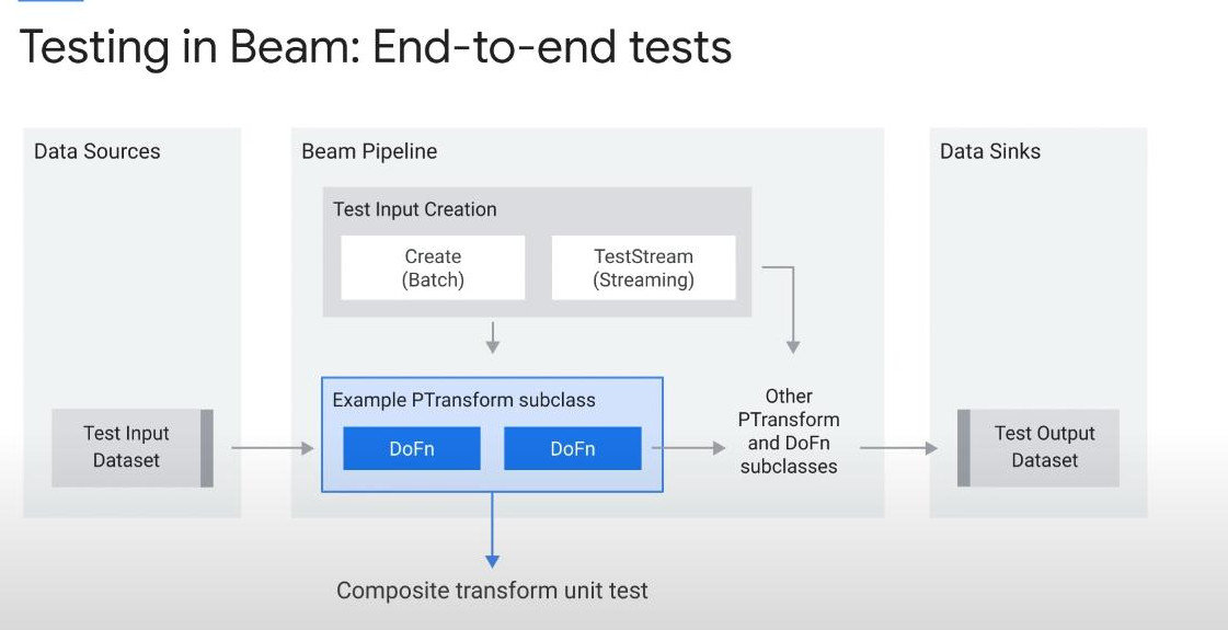
        • Common tasks for DirectRunner and ProductionRunner:

          • DirectRunner: local development, functional unit tests, small/medium integration tests.
          • ProductionRunner: medium/large integration tests, performance test, deployment/rollback testing.

        • CI/CD life-cycle:

          • Development -> Build & Test -> Deliver & Deploy.

      • Unit testing:

        • We use unit test to assert behavior of any small testable piece of our production pipeline. This small portions are either individual DoFns or PTransforms.

        • Unit test should complete quickly and can run locally with no dependencies on external systems.

        • Beam uses Junit 4 for unit testing in Java SDK, and beam.testing in Python SDK:

        • We use TestPipeline in place of Pipeline when we create a pipeline instance for testing because we can handle “setting pipeline options” internally with TestPipeline.

        • For assertion on the contents of PCollections, we use assert_that despite of which runner are used, DirectRunner or DataflowRunner. We also have

        from apache_beam.testing.test_pipeline import TestPipeline
        from apache_beam.testing.util import assert_that, equal_to, greater_than_or_equal_to, less_than_or_equal_to
        
        p = TestPipeline(desc="pipeline for testing")
        
        (p  | 'Create' >> beam.Create([1, 2, 3])
            | 'AddOne' >> beam.Map(lambda x: x + 1)
        )
        
        assert_that(result, equal_to([2, 3, 4]))
        
        ## Test if all output values are >= [2, 4, 6]
        
        assert_that(output, greater_than_or_equal_to([2, 4, 6]))
        
        ## Test if all output values are <= [10, 8, 6]
        
        assert_that(output, less_than_or_equal_to([10, 8, 6]))
        
        

        • Anti-Pattern that we should not use in our pipeline because it is a challenge to test:

          • Anonymous DoFns: ones that has no name like when we use lambda. Solution is to name it.

        • Named subclasses are easily testable so we validate its behavior independently without having to execute the entire pipeline.

        • We can test window behaviors with beam.window.TimestampedValue()
        • We can test the entire pipeline with TestStream()

      • Integration testing:

        • Small integration test: create a small amount of data for testing

        • Large integration test: carry out the test on data that is closer to production-scale. We can clone data from production project to testing project.

        • “Storage Transfer Service” to clone. It can copy a BigQuery dataset or even a read_only Production dataset.

        • In integration test, we typically test the entire pipeline without sources and sinks, meaning we can create an input data and assert the ouput of the pipeline transformations matches our expected result.

        • Testing Streaming Pipelines from PubSub:

          • To clone the Pub/Sub stream, just create a new subsription against the production topic. Then we integrate it to a testing pipeline that has passed unit testings. After that, comparing the outputs of the two pipelines Production and Testing for assertion of this integration test:

          

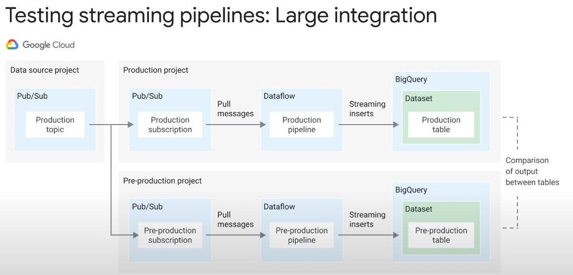
          • We should do this integration testing in a regular cadence, especially after we have had a certain amount of minor updates.

      • Artifact building:

        • Semantic version of Beam is under pattern of Major.minor.incremental
          • Major versions are incremented for incompatible API changes.
          • Minor versions are incremented for new functionality in a backward incompatible manner.
          • Incremental versions are incremented for forward compatible bug fixes.

      • Deployment:

        • 3 stages of the pipeline lifecycle: Deployment - In-flight - Termination

        • Deployment: 2 ways:

          • Direct launch : via gcloud commands
          • Use Templates : such as via Airflow

        • Separating between development environment and execution environment would make it easy to automate our Dataflow deployments.

          • External scheduler like Airflow, which actually invoke a template as deployment.
          • Each pipeline will have a unique name for Dataflow to identify, manage and monitor.

        • In-flight pipelines: only for streaming, what actions that can or shouldn’t be taken during running pipeline:

          • Dataflow manage states to eliminate the risk of data loss. It control states via snapshots.
          • Since streaming pipeline is always running, we have to modify from time to time, so we can do this safely by using snapshot to store specific states of a pipeline.

          • Snapshot saves currently executing pipeline before launching a new pipeline. This way, we can rollback to the previous version by the snapshot.

          • Snapshot functionality for certain use cases:

            • Being a checkpoint to roll back our pipeline in the event of bad release.
            • For backups and recovery.
            • A safe path for migrating pipelines to Streaming Engine. This means we can run a job directly from a snapshot on a streaming engine service, not Dataflow itself. Therefore, this process requires streaming engine service enabled.

          • Snapshot creation: we can create a snapshot in the UI or using CLI.

            • In the UI: press the “CREATE SNAPSHOT” button at the top.
            • The pipeline will pause processing while the snapshot is being built up.
            • Snapshots should be taken daily or on a weekly cadence when latency can be tolerated such as non-buiness hours.

          • Create a job from a snapshot:

          • Update a pipeline: only after taking a snapshot.

            • Why: improve performance, fix bugs, or just make necessary changes.

            • Two must options that we must add as updating a pipeline:

              • –update
              • –jobname=”current_existing_name” (_must use old name otherwise it fails to replace the old pipeline)
              • –transformNameMapping=’{“oldTransform1”:”newTransform1”, “oldTform2”:”newTform2”}’ (in case of changing 2 transforms names 1 & 2)

              python ... --update --job_name="current_existing_name"
              

            • Note: new transforms may or may not take effect, depending on where the records are buffered.

            • Updates can also be triggered via the API, enabling continuous deployment contingent on other tests passing.

            • Compatibility Check: Dataflow will check compatibility on any changes we made to the pipeline. Compability check will fail in some cases:

              • Modify without “a transform mapping”: if we renamed or removed any steps, we need a transform to map data between its two adjacient steps. It is important intermediate data can be fully processed.
              • Adding/removing side inputs: because it will change the input schema. Just recall that Dataflow always treats side input as an independent object.
              • Changing coders (or different data encoding)
              • Switching locations: new zone or new region

              • Removing stateful operations: remove any state-dependent operation in a Fusion, the check will fail.

              • NOTE: if any changes that fails the compatibility check is required, we should drain our pipeline, then rerun the pipeline with the updated code.

        • Termination: 2 ways to terminate our pipeline.

          • Drain (only for streaming): stop data input and process all buffered intermediate data. After that, the pipeline is torn down.

          • Cancel (both batch and streaming): cease all data processing and drops any intermediate, unprocessed data.

          • Press “STOP” button on the top of the Dataflow UI, we will have 2 options: “drain” or “cancel”.
            • Drain drawbacks: incomplete aggregations will happen because all windows will be closed immediately. Solutions: We can use Beam PaneInfo to recover incomplete windows as everpane is implicitly associated with a window.
            • Cancel drawbacks: intermediate data will be lost.

        

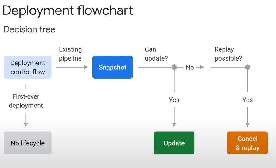
    • Reliability (Độ ổn định): When a pipeline fails, what will be lost and who is responsible for this loss. Those are the things “Reliability” will cover.

      • Loss:

        • For batching: data is not lost, just rerun the pipeline.
        • For streaming: data engineer must act fast to minimize data loss and downtime.

      • Failures:

        • User code, data shape such as software bugs or corrupted data.
        • Outages: service outages (), zonal or regional outages.
      • Monitoring:
        • Batch: a failed task will be retried 4 times.
        • Streaming: a failed task will be retried indefinitely, making pipeline stall indefinitely.
      • Solution:
        • Implementing a Dead-letter sink in a upstream ParDo using a Try-Except block.
        • Monitoring and Alert policies should be applied. Potential metrics to alert on:
          • Job status:
          • Elapsed time: if it exceeds a threshold, alerting
          • Data freshness: so high not good
          • System latency:
          • Your custom metrics if necessary.

    • Flex Templates

26. Data Mesh and Dataplex:

    1. Dataplex: is a data fabric and data governance service that allows you to organize, manage, and secure data across GCP (BigQuery, Cloud Storage, etc.) — all without moving the data.

       • Dataplex hierarchy: dataplex instance -> lake instance(s) -> zone instance(s) -> asset instance(s). Each asset could link to a data source (bucket, table…).

       • Unified Data Management: Dataplex lets you group related datasets (e.g., BigQuery tables, GCS buckets) into logical data domains (called “lakes” and “zones”).

       • Metadata and Discovery: Automatically captures metadata (schema, classification, profiling). Makes it easier to search, catalog, and understand data across the platform.

       • Data Governance & Security: Policies can be centrally defined and enforced (e.g., role-based access, data classification). Helps ensure data compliance.

       • Serverless Data Quality & Monitoring: Supports data profiling, validation, and monitoring jobs.

       • Integration with Data Tools: Works with BigQuery, Dataproc, Cloud Storage, and Data Catalog. Enables automated Spark jobs and serverless data exploration via notebooks.

       • Data Lakehouse Foundation: Helps unify batch and stream processing from raw to curated data. Supports the lakehouse architecture: raw data in GCS + refined data in BigQuery.

    2. Tagging a dataplex asset(based on Cloud Catalog): in Dataplex UI, select “Catalog” then “Create Tag Template”… . It’s like using tag to filter out a specific information from the assets (for ex: some columns in certain tables). Creating by entering Manage Metadata in Dataplex UI.

    3. Security or adding role/rights to a user: In Dataplex UI, click on “Secure” tab and expand the project-id to see the “Asset”, click on it, then “grant access” btn, paste user email on “New principal” then select a role (reader or writer) we want to grant to them. This shows the power of Dataplex on data security governance.

    4. Data Quality (based on Dataproc): In Dataplex UI, choose “Process” to set a task to validate the quality of data. The validation specification is set by .yaml file (always complicated). We have to choose a dataset to store the result. Inside the final of result table, there will be a query used for validation (but it’s very long and complex.)

27. 10 common questions for a data engineer:

    1. (1)What is the difference between ETL and ELT?:

       • ETL is traditional pipeline where we extract, then transform data before loading to cloud:

         • Cost-efficient because we don’t store raw data on cloud
         • Transformation is processed locally so we might need a strong local computer.
         • Best for sensitive data when we need strict control over transformation logic before ingesting our data to cloud.
         • It can take more time and money if we want to change transformations.
         • Tools: Apache NiFi, Talend, Informatica.

       • ELT is new with transformation is handled on cloud after loading and extracting.

         • Cost more to store raw data on cloud but transformation now can be flexible.
         • Transform queries in Bigquery also increase the cost but we can mitigate it with partitioning, clustering and materialized views.
         • Fit better for streaming because transformation can only happen in cloud.
         • CI/CD and Unit testing is easier because of most of our transformation code is available on cloud for all testers.
         • Tools include dbt, Dataform, BigQuery SQL scripts.

    2. What is “schema drift ?”

       • Schema change during streaming, new column appears.
       • Handle “schema drift” without stopping our pipeline.
       • 2.1 use “auto-detech schema” feature of Bigquery, this won’t break up our stream.

       • 2.2 Within pipeline, we can code to accept ‘new column’ and give some alert if stricter like below:

         for key, value in record.items():
             transformed[key] = value  # Copy all fields blindly
         
         known_fields = get_current_schema_fields()  #list of allowed field names
         for key in record:
           if key in known_fields:
             transformed[key] = record[key]
           else:
             log.warning(f"Unexpected field: {key}")
         
         # we should periodically to check the known_fields.
         

       • 2.3 Maybe we can code to tolerate an optional column that we know it sometimes disappear like the ‘device’ column below:

         class ParseEventFn(beam.DoFn):
           def process(self, element):
             # Decode JSON
             record = json.loads(element)
         
             # Common fields (exist in both v1 and v2)
             user_id = record['user_id']
             event_type = record['event_type']
         
             # Optional v2 field
             device = record.get('device', None)  # Handle missing field safely
         
             yield {
                 'user_id': user_id,
                 'event_type': event_type,
                 'device': device                 # Will be None for v1
             }
         

       • 2.4: Use metrics to monitor schema:
         • Filter by job and counter: calculate number of columns in the schema.

       • 2.5: Set an alert on threshold:

         • Schema evolution just happened.
         • More than 10 unexpected fields in a window.
         • A specific critical field like user_type suddenly appears.

         from apache_beam.metrics.metric import Metrics
         
         class SchemaDriftDetector(beam.DoFn):
             def __init__(self):
                 self.extra_fields_counter = Metrics.counter(self.__class__, 'extra_fields_detected')
                 self.missing_fields_counter = Metrics.counter(self.__class__, 'missing_fields_detected')
                 self.total_columns_metric = Metrics.distribution(self.__class__, 'input_column_count')
         
             def process(self, element):
                 # Decode JSON row
                 record = json.loads(element)
                 incoming_fields = set(record.keys())
         
                 # or load from config
                 expected_fields = {'user_id', 'event_type', 'timestamp'}
         
                 # Count how wide the event is
                 self.total_columns_metric.update(len(incoming_fields))
         
                 # Detect new/extra fields
                 for field in incoming_fields - expected_fields:
                     self.extra_fields_counter.inc()
                     logging.warning(f"Extra field: {field}")
         
                 # Detect missing fields
                 for field in expected_fields - incoming_fields:
                     self.missing_fields_counter.inc()
                     logging.warning(f"Missing field: {field}")
         
                 yield record
         
         # So, we have thress custom Metric names that are perfect for alerting:
         # "input_column_count"	Distribution of how many fields each record has
         # "extra_fields_detected"	Count of new/unexpected fields in current records
         # "missing_fields_detected"	Count of expected fields that are absent
         

    3. How to keep idempotency in streaming? = how to avoid duplication issue while streaming?

       • Any step in pipeline may fail and be retried, so it can send one record over one times. In streaming, duplication can happen due to: Pub/Sub retries, network retries, application retries (restart).

       • As windowing, beam.Distinct() will remove deduplicates by key within each window. This requires the upstream source (before Pub/Sub) to add event_id to each record

       | "Window into 5 minutes" >> beam.WindowInto(FixedWindows(300))
       | "Deduplicate" >> beam.Distinct(lambda row: row['event_id'])  # Based on event_id
       

       • A trade-off of beam.Distinct() is duplication could still happen in different windows, so we can extend windows longer or applying scheduled query to upsert in Bigquery.

       MERGE target_table AS T
       USING staging_table AS S    # pipeline output
       ON T.event_id = S.event_id
           WHEN MATCHED THEN
               UPDATE SET T.value = S.value, T.updated_at = CURRENT_TIMESTAMP()
           WHEN NOT MATCHED THEN
               INSERT (event_id, value, created_at)
               VALUES (S.event_id, S.value, CURRENT_TIMESTAMP())
       

    4. Dead-letter queue (DLQ) is what and how side-ouput can handle it:

       • A dead-letter queue is a storage where unprocessable records are sent instead of breaking the pipeline. The common number of retrying to process is set in a subscription. If we dont handle these bad records properly, our pipeline can get crashed.
       • Side-output is used to handle it:

       class ProcessRecord(beam.DoFn):
       def process(self, element):
           try:
               cleaned = parse_json(element)
               yield cleaned  # main output
           except Exception as e:
               yield beam.pvalue.TaggedOutput("dead_letter", {
                   "original": element,
                   "error": str(e)
               })
       
       # Then you use it like this in the pipeline:
       results = p | beam.ParDo(ProcessRecord()).with_outputs("dead_letter", main="valid")
       
       valid_data = results.valid  # continue as normal
       invalid_data = results.dead_letter  # inspect later
       

       • Cloud Storage is usually a place to store “dead-letter” data, then we can use BigQuery to analyze if it is complicated.

    5. Retry strategy to handle failures of calling external APIs:

       • we can set the number of retries for calling an external API, it’s a best practise a data engineer should do like the following snipet:

         import apache_beam as beam
         import requests
         import time
         
         class CallExternalApiDoFn(beam.DoFn):
           def __init__(self, max_retries=3, delay=1):
             self.max_retries = max_retries
             self.delay = delay
         
           def process(self, element):
             url = f"https://example.com/api/data?id={element}"
             attempts = 0
         
             while attempts < self.max_retries:
               try:
                 response = requests.get(url, timeout=5)   # 5s for a response to come out
                 response.raise_for_status()  # raises HTTPError for 4xx/5xx
                 yield response.json()        # successful result
                 return
               except requests.exceptions.RequestException as e:
                 attempts += 1
                 if attempts >= self.max_retries:
                   yield beam.pvalue.TaggedOutput('failed', {
                       'id': element,
                       'error': str(e)
                   })
                 else:
                   time.sleep(self.delay)  # wait 1s before retrying
         
         
         # in beam pipeline:
         results = (pipeline
         | 'Create IDs' >> beam.Create([1, 2, 3])
         | 'Call API' >> beam.ParDo(CallExternalApiDoFn()).with_outputs('failed', main='success')
         )
         
         results.success | 'Print Success' >> beam.Map(print)
         results.failed  | 'Print Failures' >> beam.Map(print)
         

    6. Fusion breaking to avoid “hot key” problem of data skew:

       • Hot key issue refers to a case when one key appears millions times more than any other keys, so all records going with that key will be sent to one worker as fusion happens, causing a bottleneck issue. We need to do a “fusion breaking” with .withFanout() family of methods.

       • break fusion by “fanout” methods, so that multiple workers can handle it. Please keep in mind that only combinePerKey(), sum, min, max, average, count() support “fanout” methods, GroupByKey, CoGroupByKey, CombineGlobally() dont support.

       | beam.CombinePerKey(my_combine_fn).withFanout(10)
       
       | beam.CombinePerKey(my_combine_fn).withHotKeyFanout(lambda key: 10 if key == "global" else 1)
       
       # assume that the hot key is "null", we need to give it a name "global"
       # If hot key is not null, and it is "admin", we do not need this below step
       
       def assign_key(record):
         key = record.get("user_id")
         if key is None:
           return ("global", record)  # Hot key bucket
         return (key, record)
       
       beam.Map(assign_key)
       

       • Under the hood, Beam splits the key into N shards, it performs partial aggregation in parallel. Then merges the results for the final combine.

    7. (2)How do you design a data pipeline for reliability and scalability? :

       • For batch:

         1. data source: upload data onto Cloud Storage (unstructured), Cloud SQL or Cloud Spanner (structured).
         2. Transforms: dataflow
         3. Data sink: Bigquery or Cloud Storage (back-up)

       • For stream:

         1. Data source: pub/sub
         2. Transforms: dataflow
         3. Data sink: Bigquery or Cloud Storage (back-up or late recordings)

       • Dataflow Reliability:

       • Serverless, if a node fails, another node will be auto added without any pipeline interuption.

       • Optimizing the pipeline graph continuously.

       • Code-based is very useful to help us to handle many issues or errors like:

         • “schema drift”:
         • idempotency: to handle duplication,
         • dead-letter: be handled by side-outputs,
         • retry strategy: to handle external API calling failures,
         • fusion breaking: to avoid “hot keys” using “fusion breaking” technique with built-in “withFanout()” methods.

       • Able to handle out-of-order data (late arriving records) with watermarking that works fully automatically, even across distributed systems with thousands of machines.For ex, if a sensor sends data late, but it happens regularly, Dataflow learns to adjust its watermark to wait a bit longer before closing windows completely.

       • Memory optimization: large memory usage can lead to higher cost, so try:

         • Use “fixed windowing” instead of sliding or session windowing because less overlapping means less state in memory.
         • Smaller Window size: too long window can overload memory.
         • Small allowed_lateness: too long allowed_lateness means longer state.
         • Less triggers: too many triggers can lead to more states to remember in memory.
         • avoid ACCUMULATING mode at triggerring: repetition at discarding mode can be very expensive. Discard mode is prefered with less memory and computation.
         • Aggregation: use combinePerKey to will combine data locally on each workers before shuffling. This will reduce the amount of data significantly compared to method GroupByKey() dont do local aggregation. Local aggregation helps shuffling happen less expensive, less data movement among nodes.

       • Monitoring: Cloud-Monitoring that allows setting custom metrics to manage pipelines properly.

       • Testing: Unit-test facility is also integrated in Dataflow

       • Dataflow Scalability:
         • Auto-scaling (horizontal): when there are more streaming data coming, more nodes are added automatically by Dataflow.

    8. (3)What are partitioning and clustering in BigQuery?: [done]

       • Partitioning: (PARTITION BY date) BQ will devide physically data into shards of data, each shard looks like a dict with date as key. So, filter by date or GROUB BY date will have faster performance, and more important less data is scanned, then reduce query cost. Please note that don’t apply partitioning a column with with high cardinality (only unique values).

       • Clustering (CLUSTER BY user_id): BQ will sort column ‘user_id’ within a partition if having, store data into “sorted blocks”, each block having same user_id. This help reduce the scanning time as filter by user_id or JOIN, less data will be scanned, reduce query cost. We can cluster up to 4 columns, but only the first is truly sorted. Please note that don’t apply clustering a column with with high cardinality (only unique values).

       • When would you use one vs both? Partioning is always the first of choice for queries of JOIN, GROUP BY or FILTER, then we can add clustering latter if necessary.

    9. (4) What’s the difference between batch and streaming processing?:

       • Batching processing:

         • Data has a fixed size which made a bounded PCollection in a pipeline.
         • Windowing can be used to optimize memory usage if data is too large.
         • Processing can be simpler because data is not time-sensitive.
         • Results are usually computed once, often on a schedule (e.g., daily, hourly)
         • Cost is predictable since the data volume is known in advance, and billing is typically calculated based on jobs that run periodically (daily, hourly).

       • Streaming :

         • Data is undefinite which made unbounded PCollection in a pipeline.
         • We need to use windowing to optimize memory usage while maintaining pipeline performance.
         • Stateful processing usually happens in streaming pipeline. States can be expensive but we can mitigate it from the designing stage such as combinePerKey, fixed windowing, small allowed lateness…
         • Processing is complex because data is time-critical. We have to use watermark and triggers to deal with out-of-order records or lateness.
         • Autoscaling is required to deal with load variations to maintain stable performace.
         • It’s better to use ELT pipeline with cloud services like Dataflow, Pub/Sub, Cloud Storage.
         • Dead letter should be applied.
         • Fraud Detection is needed in some cases.
         • Cost increases in time-line so that real-time report or minitor is neccesary.

    10. (5)How do you handle slowly changing dimensions (SCD) in data warehousing? :

        • Types of SCDs: There are several types of SCDs, with the most common being:

          • Type 1 (Overwrite): The new data overwrites the old, and no history is kept. This is simple but loses historical information.

          • Type 2 (Full History): When a dimension attribute changes, a new record is created with a unique identifier, and the old record is marked as historical. This provides a full history of changes.

          • Type 3 (Limited History): Limited history is tracked, often by adding new columns to the dimension table to hold previous values for specific attributes.

        • SCDs are crucial for accurate reporting and analysis, show how data evolved over time, which can be valuable for understanding trends and making decisions.

        • Practical examples (e.g., customer address changes): based on how addresses influence customers’ demand, we can make decision to apply the SCD type in our data.

          • If we sell skin care products: I think we can choose type 2, because address might show financial level of a customer and our products cycle are short, so address is really important for our business analysis.
          • If we sell books: I think we can choose type 1, because address does not hold an important position with bying a book.
          • If we sell cars: we can choose type 3, because address is important but the time for a customer to change a car is long, so maybe we just need two addresses.

        • SQL: we can use features is_current, valid_from/valid_to to add details to address status while MERGE 2 tables of different years with different addresses based on type 2:

          MERGE INTO customers_history AS target
          USING staging_customers AS source
          ON target.customer_id = source.customer_id AND target.is_current = TRUE
          
          WHEN MATCHED AND target.address != source.address THEN
            UPDATE SET target.is_current = FALSE, target.valid_to = CURRENT_DATE()
          WHEN NOT MATCHED THEN
            INSERT (..., is_current, valid_from )
            VALUES (..., TRUE, CURRENT_DATE() )
          

    11. (6)What is schema evolution, and how do you handle it?: Number 2 about “schema drift”

    12. (7)What are common causes of data quality issues & how do you detect them?:

        • Nulls, duplicates, invalid types, stale data, broken joins are data quality that we need to check. Tools that we can use:

        • Dataform with expect(): used to validate data — such as checking for nulls, duplicates, or invalid formats — and can be integrated into CI/CD pipeline to fail a deployment if data quality checks don’t pass:

          # Check for valid email format:
          expect("valid_email_format", `
          SELECT *
          FROM table_name
          WHERE NOT REGEXP_CONTAINS(email, r'^[^@]+@[^@]+\.[^@]+$')
          `);
          

        💡Fails if any email does not match the pattern

        # Check for duplicate IDs
        expect("no_duplicate_customer_ids", `
        SELECT customer_id, COUNT(*)
        FROM table_name
        GROUP BY customer_id
        HAVING COUNT(*) > 1
        `);
        

        💡Fails if any customer ID appears more than once

        
        - Dataplex task of data quality:
        - Scheduled SQL validations:
        
          ```sql
          SELECT *
          FROM users
          WHERE NOT REGEXP_CONTAINS(email, r'^[^@]+@[^@]+\.[^@]+$');
        
          # Send alerts (e.g., via Slack, email, or monitoring dashboards)
        

    13. (8)How do you optimize performance and cost in BigQuery?:

        • Use partitioning, clustering: used to reduce scanned data considerably while filter, group or join (check more at number 8).

        • Materialized views: Bigquery will save “materialized view” permenantly and auto refreshed and updated from the source table. Materialized View can improve signigicantly ther performance of workloads because of its caching results. (note: storage cost will arise for “materialized view”). If we use “With clause” so many times, “Materialized view” will be a effective way to improve queries performance because “with clause” is not cached like “Materialized view”.

        • Query pruning: we have some common types of pruning:

          • partition pruning: we only filter exactly partitioned column
          • cluster pruning: we only filter exactly clustered column
          • Column Pruning: SELECT customer_id FROM users, it is faster because it will only read one column ‘customer_id’ because BQ_table is columnar.

        • Avoid “SELECT *”: even with filter or limit N, “select *” still scan all the data so that it is slow and very expensive in most case, we should always select specific columns as a best practise.

    14. (9) What’s the difference between a data lake, data warehouse, and data lakehouse? [done]

        • Datalake: store raw, uncurated data in formats like JSON, CSV, Parquet, images, and videos (structured + unstructured). It is used for data science. Example is Cloud Storage.

        • Warehouse: processed data with structured format, used for business analysis. Example is Bigquery. Both SQL-based query and AI tools are supported.

        • Lakehouse: a combination of datalake plus warehouse for overal governance in one place. It automatically captures metadata (schema, classification, profiling) without moving it, making it easier to search and understand data across many sources in cloud. Dataplex is a tool to build a lakehouse.

    15. (10)What makes a pipeline “production ready”?:

        • Monitoring: set up monitoring strategy for critial parameters.
        • alerting: define thresholds a pipeline parameters cannot pass.
        • retries: handle external API with a suitable retries strategy.
        • testing: Unit test for functioning and integration testing with small data to assure stability using DirectRunner of Dataflow.
        • documentation: a general description of the pipeline: input type, which transformation, expected outputs.
        • versioning: use Git to store and manage versions of the pipeline
        • CI/CD: applied small testing as pushing or updating (new) features
        • data quality checks: build a lakedata UI to monitor data quality and Dashboard if necessary.

Share on:

• Twitter
• Facebook
• Reddit