Bq Sql Highlights

Traininng and training more in different contexts:

WHERE state IS NOT NULL AND state <> ‘’ : gives a note that “null is not a blank”.
SESSION_USER() AS viewer is a func to call out “the current session loginned user”.
WHERE REGEXP_EXTRACT(SESSION_USER(), r’@(.+)’) IN (‘qwiklabs.net’) : not filter but check out the current session loginned-user permission to be allowed to see the data.

How to create a VIEW with an expiration in BQ:

 CREATE OR REPLACE VIEW ecommerce.vw_large_transactions
 OPTIONS(
 description="large transactions for review",
 labels=[('org_unit','loss_prevention')],
 expiration_timestamp=TIMESTAMP_ADD(CURRENT_TIMESTAMP(), INTERVAL 90 DAY)
 )
 AS

WHERE date BETWEEN ‘2020-04-01’ AND ‘2020-04-30’ just a datetime filteration.
WHERE date IN (‘2020-02-21’, ‘2020-03-14’) : just another datetime filteration.

Compare cumulative_confirmed_cases between 2 adjacent rows (or dates):

 LAG(cases) OVER(ORDER BY date) AS previous_day,
 cases - LAG(cases) OVER(ORDER BY date) AS net_new_cases

Compare cumulative_confirmed_cases between 2 adjacent rows (or dates) in percentage:

 LAG(cases) OVER(ORDER BY date) AS Cases_Previous_Day,
 CASE 
   WHEN LAG(cases) OVER (ORDER BY date) IS NULL THEN 0
   ELSE (cases - LAG(cases) OVER (ORDER BY date)) * 100 / LAG(cases) OVER (ORDER BY date)
 END AS Percentage_Increase_In_Cases

LAG(cases) OVER(ORDER BY date) AS Cases_Previous_Day : is a way to call the previous row.
LEAD(total_cases) OVER (ORDER BY date) AS last_day_cases is a way to call the next row.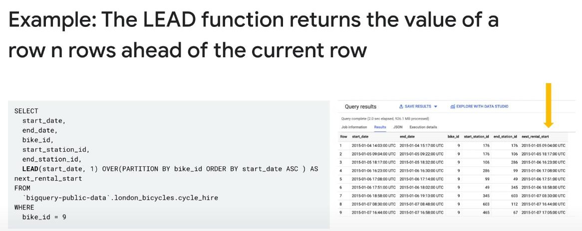
DATE_DIFF(LEAD(date) OVER(ORDER BY date), date, day) AS days_diff : is a way to find out the numeric difference between “current date” and “next date”.
- Other case using ‘DATE_DIFF(1, 2, 3)’
  - DATE_DIFF(CURRENT_DATE(), date, DAY) AS partition_age,
POWER(a, b) AS cdgr :

Could we “select” data FROM 2 tables at the same times: (make sure that they have the same number of rows, maybe 1 rows better)

SELECT
  total_visitors,
  total_purchasers,
  total_purchasers / total_visitors AS conversion_rate
FROM visitors, purchasers

ROUND(SUM(Revenue/1000000), 2) AS revenue

a way to reduce the number of “decimal digits” in the long float number 1.12345679183488093274

SELECT * EXCEPT(fullVisitorId) FROM… : could be like that??

UNNEST() : equal to flatten() a nested object.

SELECT p.v2ProductName,
FROM `data-to-insights.ecommerce.web_analytics`,
UNNEST(hits) AS h,
UNNEST(h.product) AS p...

Simply: p.v2ProductName = hits.product.v2ProductName => no need UNNEST().

IFNULL(totals.bounces, 0) AS bounces, set NULL to 0.
- IFNULL(geoNetwork.country, “”) AS country :

Call out a ROC as evaluating a model:

SELECT
  roc_auc,
  CASE
    WHEN roc_auc > .9 THEN 'good'
    WHEN roc_auc > .8 THEN 'fair'
  ELSE 'poor' END AS model_quality
FROM
  ML.EVALUATE(MODEL ecommerce.classification_model, ...input_data_table...)

MAX(CAST(h.eCommerceAction.action_type AS INT64)) AS latest_ecommerce_progress : we also have MAX() function.

How to creat a new model in BigQuery:

CREATE OR REPLACE MODEL `ecommerce.classification_model`
OPTIONS (
  warm_start = true,
  model_type='logistic_reg',
  input_label_cols = ['will_buy_on_return_visit'],
)
AS ...input_table...

How predict in BigQuery:

SELECT *
FROM ml.PREDICT(MODEL `ecommerce.classification_model_2`, ...input_table...)

select TIMESTAMP_TRUNC(pickup_datetime, MONTH) month, : extract only the month but keep pickup_datetime format unchanged in the result like 2015-01-12 00:00:00 UTC, not 01.
select EXTRACT(HOUR FROM pickup_datetime) hour, : now literally extract only the time and forget the pickup_datetime like 0 or 23 h.

SELECT [‘Sun’, ‘Mon’, ‘Tues’, ‘Wed’, ‘Thurs’, ‘Fri’, ‘Sat’] AS daysofweek

build a list, thereafter we could call daysofweek[0] => Sun.

Use “WITH” to build a table ‘tA’ to contain this list then add it to “FROM table, tA”.

select EXTRACT(DAYOFWEEK FROM pickup_datetime) : extract 0-6 with 0 as Sunday.
MOD(17, 1000) : take the remainder after a division.

FARM_FINGERPRINT()

Generates a deterministic 64-bit hash value for the input string with a rule, always generating the same hash with same input,

How to create model with linear_reg:

CREATE or REPLACE MODEL taxi.taxifare_model
OPTIONS (model_type='linear_reg', labels=['total_fare']) AS
      WITH params AS (
        SELECT 
          1 AS TRAIN,
          2 AS EVAL
        ),

      taxitrips AS (
        SELECT ... 
        FROM ...
        WHERE
          trip_distance > 0 AND fare_amount > 0
          AND MOD(ABS(FARM_FINGERPRINT(CAST(pickup_datetime AS STRING))),1000) = params.TRAIN
      )

      SELECT *
      FROM taxitrips

params.TRAIN : for training (rule of BQML)
params.EVAL : for evaluation

STDDEV(fare_amount) AS stddev : standard deviation in SQL.
ORDER BY season # default is Ascending (low to high) : default is “ASC”

IF(COUNTIF(totals.transactions > 0 AND totals.newVisits IS NULL) > 0, 1, 0)

if user is “not a new user” and buy something, give out “1”.

COALESCE(first, second, …, n_exp, 0) : from left to right, which not NULL will be shown.
APPROX_QUANTILES(tripduration, 10)[OFFSET (5)] AS typical_duration : an aggregate function to devide “all tripdurationS = array” into 10 parts, and take the number of the “5th boundary”.

Calculate the distance by geographical points with ST_Distance() and ST_GeoPoint()

ST_Distance(
  ST_GeogPoint(s.longitude,s.latitude),
  ST_GeogPoint(e.longitude,e.latitude)) AS distance

How to check all tables in a dataset:
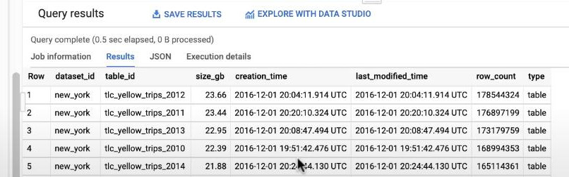
- FROM project_id.dName.__TABLES__ will fetch all tables in dataset ‘dName’.
- SELECT dataset_id, table_id will extract the name of dataset & table.
- SELECT size_bytes, row_count, type will extract the size, number of rows, type (1 means Table, 2 means View). (we should change size_bytes to GB by dividing by 10^9, then rounding to 2 decimals).
```
  CASE 
  - WHEN type=1 THEN 'table' 
  - WHEN type=2 THEN 'vew'
  ELSE NULL
  END AS type
```
- SELECT timestamp_millis(creation_time) t1, last_modified_time t2 : will show time of creation and the latest mofification, ‘timestamp_millis()’ convert a float time to std UTC time.
How many columns and their infos of all tables in a dataset ‘dName’:
- FROM project_id.dName.INFORMATION_SCHEMA.COLUMNS
- Other feature like ‘is_partitioning_column’, ‘’
Can you find 10 tables with highest number of rows in all datasets.
```
SELECT * FROM project_id.dName1.__TABLES__ UNION ALL
SELECT * FROM project_id.dName2.__TABLES__
```
- First, we need to combine all the tables together into one table with ‘WITH’, then just filter with ORDER row_count DESC.
How to quick check all metadata of all datasets in your project:
```
FROM `project_id.INFORMATION_SCHEMA.SCHEMATA` AS s
LEFT JOIN `project_id.INFORMATION_SCHEMA.SCHEMATA_OPTIONS` AS so
USING (schema_name)
    
WHERE so.option_name = 'description'
```
- We need extract 2 schema objects ‘SCHEMATA’ & ‘SCHEMATA_OPTIONS’. Filter out the property ‘option_name’ with WHERE so.option_name = ‘description’. Note: we could see a project also has its own INFORMATION_SCHEMA.
How to use a STRUCT or ARRAY in a query.
- A STRUCT in BigQuery is a nested data type that groups multiple fields together, similar to an object in JSON or a row in SQL.
- It helps reduce ‘shuffled Bytes’ and ‘Slot time consumption’, sometimes it help reduce the bill of memory usage for a query because we have to denormalize tables to obtain STRUCTS. (denormalization: 2 tables with many similar columns -> 1 table with STRUCTs inside.)
A Normal query with JOIN and without STRUCT
```
FROM `projectID.datasetA.blocks` as b  
JOIN `projectID.datasetA.transactions` as t USING(block_id)
, t.inputs as i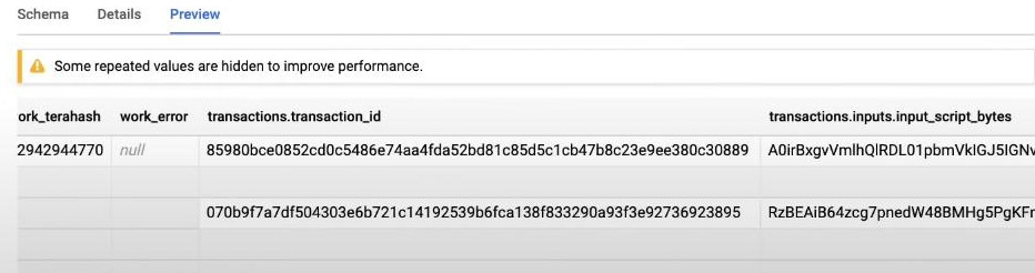  
```
A query with a STRUCT inside and without a JOIN. It reduce dramatically ‘shuffled Bytes’ and ‘Slot time consumption’. Because, luckily the table ‘blocks’ has a Struct ‘transactions’ inside by denormalization already.
```
FROM `projectID.datasetA.blocks` as b  
, b.transactions as t   -- "CROSS JOIN" a struct type
, t.inputs as i         -- "CROSS JOIN" a struct type
```
- This is benefits of a STRUCT: ‘totals.’ (looks like *flattening)
```
SELECT
  visitId,
  totals.*,
  device.*
```
- Notice
- shuffle rows means Bigquery has to visit one row many times. In this query below, Bigquery has to check all remaining rows with each user_id. This causes slow performance. We can do partitioning the user_id or filter data before aggregation with group_by or using special function “APPROX_COUNT_DISTINCT()”:
```
SELECT user_id, COUNT(*) FROM event_logs GROUP BY user_id;
```
- Slot time consumption: slot means “node” or “computing resources” used to process a query. The unit slot-seconds. In particular, if we have 100 slots, each run 5sec, => the Slot time consumption is 500 slot-seconds. Bigger table, the more slots we need. For ex, the following query will causes “high slot time consumption” if it’s not partitioned because Bigqiery has to scan all the huge table. But if the table is partitioned by event_date, BigQuery will scan only one partition => low slot time usage.
```
SELECT * FROM huge_table WHERE event_date = '2024-03-01';
```
- Besices partitioning, other optimizations are to avoid SELECT * FROM… or use “BI engine” that runs everything in-memory instead of always scanning Bigquery storage.
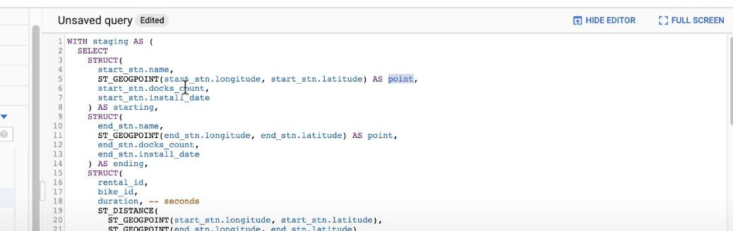
- How to create a STRUCT: (we will have a Struct-typed “starting”, we’ll have starting.name, starting.point, …)

Why use ‘UNNEST()’ : because cannot use 2 times nested query (with 2 dots): t.objA.featureb because there are more than ONE values at the first nested t.objA.

SELECT t.objA.featureb   --2 times nested query
FROM project.dataset.block_id as b,
, b.transactions as t
, t.inputs as i

Add more UNNEST(t.objA) as t_objA

SELECT t_objA.featureb   --2 times nested query
FROM project.dataset.block_id as b,
, b.transactions as t
, t.inputs as i
, UNNEST(t.objA) as t_objA

Recap: UNNEST() brings the array elements back into rows.

How to create ARRAYs in a query: (we need: ‘GROUP BY’)
```
ARRAY_AGG(v2ProductName) AS products_viewed,
...
GROUP BY date
```
- ARRAY_LENGTH(ARRAY_AGG(v2ProductName)) AS length, : bonus to ‘array_length()’
- ARRAY_AGG(DISTINCT v2ProductName) AS products_viewed, : bonus to de-duplicate
- *ARRAY_AGG( ORDER BY )* : ordering elements with
- *ARRAY_AGG( LIMIT 5)* : Limiting

How to create a STRUCT in a query:

#standardSQL
SELECT STRUCT("Rudisha" as name, [23.4, 26.3, 26.4, 26.1] as splits) AS runner

How many ways to create a SCHEMA:

in BigQuery UI as creating a new table: (hints: Edit as text)

[
 {
     "name": "race",
     "type": "STRING",
     "mode": "NULLABLE"
 },
 {
     "name": "participants",
     "type": "RECORD",
     "mode": "REPEATED",
     "fields": [
         {
             "name": "name",
             "type": "STRING",
             "mode": "NULLABLE"
         },
         {
             "name": "splits",
             "type": "FLOAT",
             "mode": "REPEATED"
         }
     ]
 }
]

Convert a String/Int64 type to DATE type:
- PARSE_DATE(“%Y%m%d”, date) AS date_formatted
- DATE(CAST(year AS INT64), CAST(mo AS INT64), CAST(da AS INT64)) AS date
Filteration techniques:
- WHERE city_name LIKE ‘D%’ starting with ‘D’
- WHERE _TABLE_SUFFIX >= ‘2021’ table_name ends greater than ‘2021’
Filter by a list: WHERE date [NOT] IN(d1, d2, d3)
Ways to deal with ‘null’: NULLIF(), IFNULL(), COALESCE()
Ways to clean string data: PARSE_DATE(), SUBSTR(), REPLACE()
What is difference between: FORMAT(), CAST()
- FORMAT(): indicate units, only return STRING type, FORMAT(1234567.89, ‘N2’) AS string_number
- CAST(): convert to new data types, CAST(123.45 AS INT) AS converted_int

Analytic Window Functions:

Standard Aggregations:

SUM
AVG
MIN
UNNEST
BIT_AND: A bit is 1 only if all numbers have 1 in that position.
BIT_OR: always keeps 1 if at least one input has 1

BIT_XOR: cancels out even occurrences of 1, keeping only odd ones.

      SELECT BIT_OR(number) AS result 
      FROM UNNEST([5, 3, 7]);

      results below
      5  →  101  
      3  →  011  
      7  →  111  
      ----------------  
      BIT_OR →  111  (result is 7)  

      5  →  101  
      3  →  011  
      7  →  111  
      ----------------  
      BIT_AND →  001  (result is 1)

      5  →  101  
      3  →  011  
      7  →  111  
      ----------------  
      BIT_XOR →  101  (result is 5)    

COUNTIF
LOGICAL_OR
LOGICAL_AND

Navigation functions:
- NTH_VALUE
- LAG
- FIRST_VALUE
- LAST_VALUE

Ranking and Numbering functions:

RANK

  SELECT name, department, start_date, 
      RANK() OVER (PARTITION BY department ORDER BY start_date) AS rank
  FROM Employees;

CUME_DISK
DENSE_RANK
ROW_NUMBER
PERCENT_RANK

With clauses: are used to define “named subqueries” that can be referenced multiple times in a query in Bigquery. It is

WITH EmployeeData AS (
    SELECT name, department, start_date
    FROM Employees
    WHERE start_date >= '2023-01-01'
)
    
SELECT name, department FROM EmployeeData WHERE department = 'IT';

Bigquery Geo Viz : a lightweight cloud application that allows for quick testing of geospatial data.
- ST_GeogPoint(longitude,latitude) is a SQL code to convert 2 FLOAT-typed longitude & latitude to a GIS-typed geospatial point (or exact coordinates - toạ độ) on GIS map (Geographic Information System) of Google.
- ST_GeogFromGeoJSON(longitudeJSON, latitudeJSON): similar to ST_GeogPoint() with JSON format.
- ST_Distance(p1, p2): distance between 2 points. (p1,p2 is GIS-typed point from ST_GeogPoint()).
- ST_MakeLine(point1, point2) will overlay a line between 2 geospatial points on a map.
- ST_MakePolygon(ST_MakeLine([point1, point2, point3])) will also overlay a triangle with 3 geospatial points on a map, helping highlight relationships in the data.
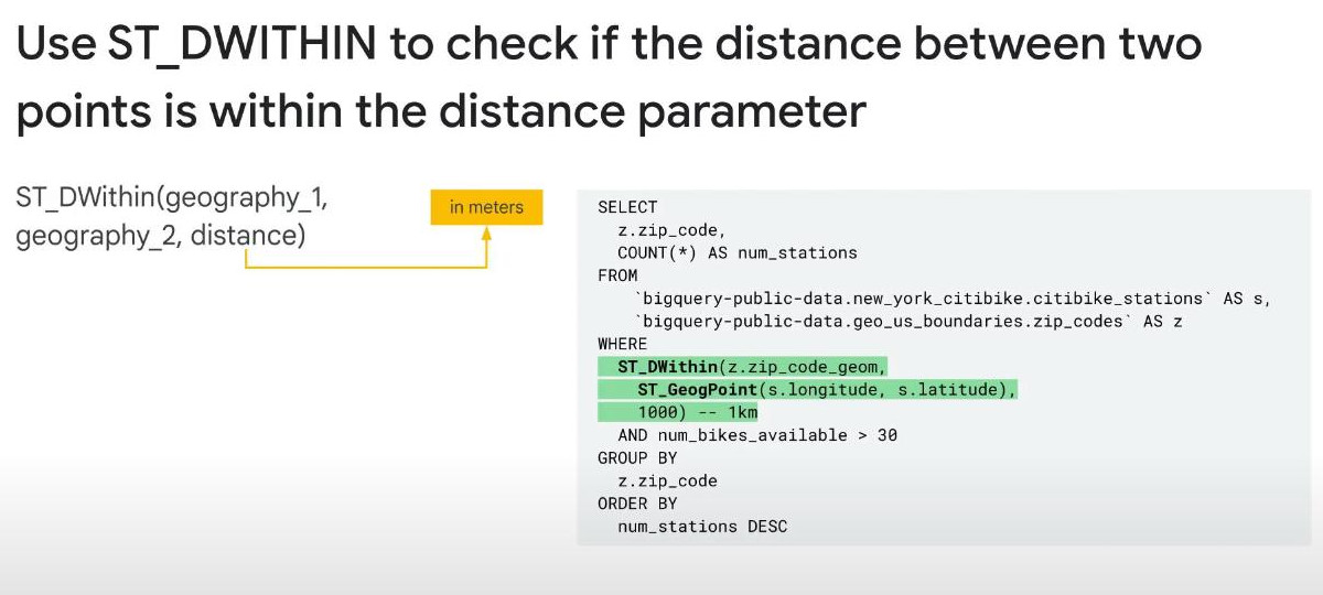
- WHERE ST_DWithin(point1, point2, 1.5e5) –150km is used to filter out bike stations (point2) within 150km linear distance from point1(a city center or the post office).
- ST_Intersets(polyA, polyB): true if two polies overlap.
- ST_Contains(polyA, point1): true if a point is inside a polygon.
- ST_ConveredBy(polyA, polyC): true if polyA is completely inside polyC.
APPROX_QUANTILES(duration, 10)[OFFSET (5)] AS typical_duration : first we have many trip durations of a rental bike, collect all the durations, sort them ASC, devive them in 10 quantiles (equal parts), select duration numbers at the edges (boundaries) of each quantiles then we will have a list of 10 numbers, because the first number has an index of 0, so the result of “OFFSET (5)” is the 5th number. (better than AVG(durations) because we can avoid skewed data)

SOFTWARE ENGINEER

Bq Sql Highlights

Share on: