Types Of Ai Architechtures

• evolution : sự tiến bộ

  innovation : sự sáng tạo

• regression : hồi quy

  classification : sự phân loại

Common Types of AI architectures:

AI technology has been “exploding” in recent years, introducing numerous new concepts and terms each year. Among these, AI architectures, in my view, play a key role in this evolution(sự tiến bộ). This post is my attempt to collect and describe some common AI architectures with their core typical features.

1. FNNs (Feedforward(truyền thẳng) Neuron Network) :

   1.1 Foundational: FNNs are the simplest neural networks and provide a foundation for understanding how inputs, weights, biases, and activations work.

   1.2 Broad Applicability: Useful for basic tasks like regression(phân tích hồi quy) and classification.

   1.3 Techniques: Basics of how neural networks process data, activation functions, loss functions, and backpropagation(truyền ngược).

   

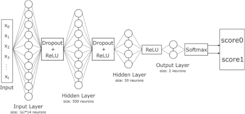
   Figure 1: regular FNN

   • Input Layer $X$: This layer receives the raw data (features or inputs). Each node corresponds to one feature of the input data.

   • Hidden Layers $H_{j}$: These intermediate layers process the input using weights and biases $W$, that are initialized randomly between 0 and 1. Each node in a hidden layer applies an activation function ReLU and regularization technique Dropout.

   • Output Layer $Y$: There are two nodes (0 & 1) at the end, so this architecture is for classification.

   For each layer with input X and output Y, we have:

   \[Y = \alpha (W \cdot X + B)\]

   With:

   • $X$: input vector
   • $W$: weight matrix
   • $\alpha$: activation function
   • $Y$: layer ouputs
     
     

   Dropout: is a regularization technique to prevent overfitting. It works by randomly “dropping out” (setting to zero) a subset of neurons in a hidden layer during each training iteration, hence these neurons have no gradient updations. This makes the network learning more generally by not relying too heavily on specific neurons.

   Notice: “dropout” sets zero forcefully to some neurons at the “forward propagation” (truyền tới), it cannot be applied at the final layer.
   
   

2. Convolutional(tích chập) Neural Networks (CNNs) :

   2.1 Complexity: CNNs are a natural progression, especially for image-related data.

   2.2 Practical Applications: Many real-world use cases (face recognition, medical imaging(2D, 3D), sentiment analysis).

   2.3 Techniques: Filters, feature maps, pooling, and convolution(tích chập) operations. These terms should be clarified to master this CNN architecture.

   

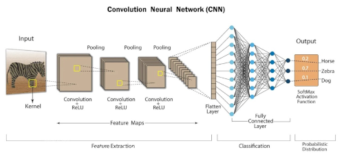
   Figure 2: Convolutional Neural Networks CNN

   

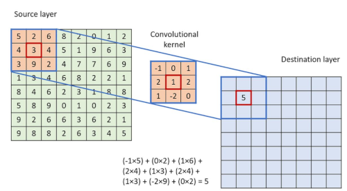
   Figure 2.1: Convolution process

   • Convolution: is a mathematical operation a kernel (a matrix or a filter) traverses over the image and performs a DOT product with each overlapping(phủ lên) areas, that is a matrix with same size. This DOT products are to extract important regional features on the image, but this is hardly understandable.

   • Filter (kernel or a matrix): There might be various filters (kernels) applied to capture various aspects of the image. The more number filters, the more features extracted or the longer the flatten layer becomes. The initial layers extract edges and texture, and the final layers extract parts of an image like head, eyes, or a tail. CNN adjusts (learns) the filters during training to minimize the loss.

   • Stride: the number of cells the kernel of filter traverse one time over the image.

   Explaination of Figure 2.1:

   • (5x-1)+(2x0)+(6x1)+(4x2)+(3x1)+(4x2)+(3x1)+(9x-2)+(2x0) = 5 (origin 3)
   • (2x-1)+(6x0)+(8x1)+(3x2)+(4x1)+(5x2)+(9x1)+(2x-2)+(4x0) = 31 (origin 4)
   • (6x-1)+(8x0)+(2x1)+(4x2)+(5x1)+(1x2)+(2x1)+(4x-2)+(7x0) = 5 (origin 5)
   • (8x-1)+(2x0)+(0x1)+(5x2)+(1x1)+(9x2)+(4x1)+(7x-2)+(7x0) = 11 (origin 1)

   After convolution calculation with stride 1, the DOT product values are scaled up as following:

   3-4-5-1 is replaced by 5-31-5-11.

   This convolution values definitely highlight the relative relationship across all the cells (pixels) in the image, improving the learning process. But as mentioned, kernel values are adjusted like “weights” during the training in most cases.

   2.4 Pooling Layers: After convolution operations, pooling takes place, which some times reduces the size of the “representation”.

   2.5 Flatten layers: is to combine and reduce the size of all the pooling layers to 1-dimentional vector feeding the next “fully connected layer” that is similar to the FNN architecture.

   • Variants: There are various types of “convolution operations”, including dilated convolution, transposed convolution, depthwise separable convolution, deformable convolution.

   2.6 Applications: tasks involving image-related data:

   • Computer Vision Applications: Image classification, Object Detection, Facial Recognition, Image Generation and Enhancement…
   • Video Processing: Action Recognition, Video Analytics, Video Segmentation.
   • Medical Imaging: MRI/CT Scan Analysis, X-ray Classification.
   • Autonomous Vehicles: Road Scene Understanding, Driver Monitoring Systems.
   • Natural Language Processing: Text Classification, Character-Level Models.
   • Robotics: Analyzing the environment.
   • Satellite and Aerial Image Analysis: Land Cover Classification.
   • Fashion and Retail: Product Recommendation, Virtual Try-On
   • Gaming and Augmented Reality: Scene Understanding, Character Animation ( Generating realistic movements based on visual data.)
   • Industrial Applications: Defect Detection, Quality Assurance
     
     

3. Recurrent(hồi quy) Neural Networks (RNNs) :

   3.1 Sequential Data: fit for time-series data, text, or speech.

   Data Flow with BTTT (Backpropagarion Through Time): it is very similar to FNNs architectures but it includes loop over time, output from previous time steps are fed back into the network as input, making the learning process will have to 2 inputs. (The feedback loop applies across the network as a whole).

   \[Y_{t} = \alpha (W_{x}X_{t} + W_{y}Y_{t-1} + B)\]

   With:

   • $X_{t}$ : normal input at time step $t$
   • $W_{x}$, $W_{y}$ : weight matrices
   • $Y_{t-1}$ : previous input at time step $t-1$

   • $\alpha$ : activation function (sigmoid, tanh, ReLU)
     
     

   • Difference: This feedback loop enables the network to maintain a form of memory, capturing “sequential dependencies” (sự phụ thuộc liên tục) in data.
   • Techniques included: Hidden states, vanishing gradients.

   
   
   

   

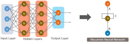
   Figure 3: Recurrent Neural Networks RNNs

   3.2 Variants: The problem with RNNs is a short-term memory that means RNNs will forget older information easily for longer sequences. Hence, LSTMs (long short-term memory) was introduced with a cell state $C_{t}$ like a memory of the network during training. $C_{t}$ is to determine what the network should forget or memorize thanks for the activation “tanh”.

   • LSTMs (Long Short-Term Memory):

   Long Short-Term Memory (LSTM) is a type of recurrent neural network (RNN) designed to handle sequential data and long-term dependencies. Its architecture includes cell states (long-term memory) and hidden states (short-term memory), regulated by three key gates: “forget, “input”, and “output”. The forget gate removes irrelevant information, the input gate adds new information, and the output gate determines the output and updates the hidden state. These gates, powered by sigmoid and tanh activations, enable LSTMs to mitigate issues like vanishing gradients, making them effective for tasks such as language modeling, time-series prediction, and speech recognition.

   
   
   

   

   Figure 3.1: Long Short-Term Memory - LSTMs .

   Cell state $C_{t}$:

   \[C_{t} = f_{t} \cdot C_{t-1} + i_{t} \cdot C^{tanh}_{t}\]

   With:

   • $f_{t} \cdot C_{t-1}$: determines how much of the previous memory to keep (or forget).

   • $i_{t} \cdot C^{tanh}_{t}$: decides how much of new information to add into the network:

   • Forget Gate (sigmoid): $ f_{t} = \alpha (W_{f} \cdot [h_{t-1}, x_{t}] + b_{f}) $

   • Input Gate (sigmoid): $ i_{t} = \alpha (W_{i} \cdot [h_{t-1}, x_{t}] + b_{i}) $

   Cell state (tanh) :

   \[C^{tanh}_{t} = tanh(W_{c} \cdot [h_{t-1}, x_{t}] + b_{c})\]

   • Ouput Gate (sigmoid): $ O_{t} = \alpha (W_{o} \cdot [h_{t-1}, x_{t}] + b_{o}) $

   • New hidden state: with added $tanh(C_{t})$, $h_{t}$ is more memorable to retain “long-term dependencies” in sequential data, such as natural language.

   \[h_{t} = O_{t} \cdot tanh(C_{t})\]

   • The output gate $O_{t}$ decides how much of the “cell state” should be passed as the “hidden state” $h_{t}$.

   • Remark: LSTMs retain information better than traditional RNNs due to their use of a “cell state” $C_{t}$ which is updated by the “forget” and “input gates”. This allows the network to maintain and regulate long-term memory more effectively.

   • Applications: while transformers dominate most NLP tasks in 2024, LSTMs remain an essential tool, especially for real-time systems:

     • Financial forecasting
     • Weather prediction
     • Predicting disease progression, monitoring patient vitals in real-time
     • Network traffic.
     • Human action recognition in videos, gesture recognition, and video captioning.
     • LSTMs are still heavily used for music generation and composition.
       
       

4. Transformer Architectures :

   4.1 State-of-the-Art: Transformers dominate modern AI applications, especially in NLP (e.g., GPT, BERT). It processes sequences in parallel rather than sequentially, using positional encodings to retain the order of inputs.

   4.2 Core terms:

   • Token: a discrete symbolic representation that are not numerical. There are more than one way of Tokenization, a token can be a word or a subword or a character. For example: [“The”, “cat”, “sat”, “on”, “the”, “mat”, “.”] is a set of tokens (words) from an input sentence “The cat sat on the mat.”.

   • Embedding: a numerical representation of a token in a continuous space. They are very dense (complex) to capture the semantic(ngữ nghĩa) relationships between tokens. For example: [0.25, 0.78, …]

   • Self-attention: a mechanism used within both the encoder and the decoder of the Transformer architecture.

   • $d_{model}$: the size of the vector representation of each token in the sequence (input data). For ex: 512 (e.g., in the original Transformer paper), 768, 1024, or larger in modern variants like BERT and GPT.

   • Techniques: self-attention mechanism, and encoder-decoder architectures.

   There are many types of Transformer models, with an input sequence “I love coding.” we could list some types based on the outputs:

   1. Translation: the transformer is trained for translation, the output should be “J’aime coder.”
   2. Text Summarization: “Passionate about coding.”
   3. Text Generation: “It’s my favourite hobby.”
   4. Sentiment Analysis (classification): output is a label “Positive”
   5. Part-of-Speech Tagging: “PRON VERB NOUN PUNCT”
   6. Masked Language Modeling: “I love coding [MASK]”, now predict “MASK” at inference but learn “coding” during training.
   7. Paraphrasing: “I enjoy programming.”

   
   
   

   

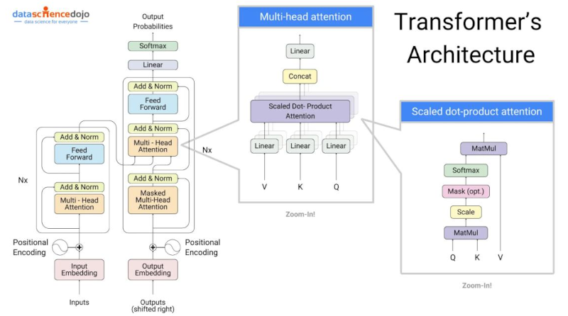
   Figure 4: Transformer Architecture

   Input Embedding ($X$) : each token in the input sequence is converted to a “vector representation”, forming a matrix $X \in \mathbb R^{n \times d_{model}}$.

   • $n$: number of tokens in the input data.

   • $d_{model}$: dimensionality of the embeddings.

   • Process of generating embeddings :
   • Each token is mapped to a vector via “an embedding layer” in the model. This layer typically involves “a learned matrix” Weights: $W_{E} \in \mathbb R^{|V| \times d_{model}}$.
   • $|V|$ : Vocabulary Size. $V$ is the “SET” of all “unique terms” (words, subwords, or tokens) that the model recognizes from the input data. If the input data only has 100 unique words, $V$ will be a dictionary or a set of 100 words, each will have a fixed index. Hence, $|V| = 100$ and each word (token) is represented by a vector (row) in matrix $W_{E}$.
   • For ex: given an input sentence “I love coding.”, via tokenization we have [I, love, coding, “.”]. Each token will have an unique index in $V$, for example, we get [1, 4, 8, 10], using these indices we could fetch vectors from $W_{E}$ to have $X = [x_{1}, x_{2}, x_{3}, x_{4}]$ with vector $x_{i} \in \mathbb R^{d_{model}}$.
     
     

   PE - Positional Encoding : Transformers lack inherent sequence information since they process input tokens in parallel. Positional Encoding (PE) provides this missing information by encoding each token’s position in the sequence.

   • Positional information is added to the embeddings using “sin” and “cos” functions, corresponding to even and odd “positions”.
   \[PE(pos,2i) = sin(\frac{pos}{10,000^{2i/d_{model}}}), \ PE(pos,2i+1) = cos(\frac{pos}{10,000^{2i/d_{model}}})\]
   • $pos$: position index of the token in “the sequence” with length n.
   • $i$: the dimension index of the embedding size $d_{model}$.
   • The final input to the Transformer is $X’ = X + PE$

   • The denominator $10,000^{2i/d_{model}}$ ensures that the positional encodings cover varying frequencies.

   • Notice: PE is fixed but the final input $X’$ is learned(changed) during training.

   Example: for a sentence sequence of 3 tokens ($n=3$), $d_{model} = 4$, we have $X \in \mathbb R^{3 \times 4}$ and $PE \in \mathbb R^{3 \times 4}$:

   \[X+PE = \begin{vmatrix} X_{0,0}+PE(0,0) & ... & X_{0,3}+PE(0,3) \\ X_{1,0}+PE(1,0) & ... & X_{1,3}+PE(1,3) \\ X_{2,0}+PE(2,0) & ... & X_{2,3}+PE(2,3) \\ \end{vmatrix}\]

   Remark:

   • One $PE$ will represent the exact position of each token in the sequence and map it into the feature vector space $\ \mathbb R^{d_{model}}$.

   Encoder Components: consists of multi-head self-attention and a feed-forward network. Self-attention is used to understand “token dependencies” (relationships between different words or phrases). Encoder stack contains $N$ identical layers. Each layer consists of:

   • 1. Multi-Head Self-Attention: It was introduced by a group of researchers at “Google Brain” in their seminal paper titled “Attention Is All You Need” in 2017. The idea is that each token in a sequence should “attend” to all other tokens (including itself), weighted by their relevance. Importantly, it allows “parallelizable computations” that improves the efficiency greatly.
   • If we have $h$ heads (8 for the first Transformer), each head will have an $attention score$ calculated in parallel:
   \[Attention_{i}(Q_{i},K_{i},V_{i}) = softmax(\frac{Q_{i} \cdot K_{i}^{T}}{\sqrt{d_{K}}}) \cdot V_{i}\]
   • Query matrix $Q_{i} = X \cdot W_{Q_{i}} $ helping the model ask “Which other words are relevant to me?”
   • Keys matrix $K_{i} = X \cdot W_{K_{i}} $ setting a label for a word.
   • Values matrix $V_{i} = X \cdot W_{V_{i}} $ holding the meaning information of a word.
   • $Q_{i}$, $K_{i}$, $V_{i}$ are 3 projections of X into 3 vector spaces in nature. $Q_{i}$, $K_{i}$ $\in \mathbb R^{n \times d_{K}}$ and $V_{i}$ $\in \mathbb R^{n \times d_{V}}$
   • $W_{Q_{i}}, W_{K_{i}} \in \mathbb R^{d_{model} \times d_{K}}$ and $W_{V_{i}} \in \mathbb R^{d_{model} \times d_{V}} $ are learnable weight matrices.
   • The “Scaled Dot-Product” $\frac{Q_{i} \cdot K_{i}^{T}}{\sqrt{d_{K}}}$ is a matrix $\in \mathbb R^{n \times n}$ represents the compatibility scores between $Q$ and $K$.
   • “Softmax” is applied along each rows to normalize the “attention scores”.
   • $X \in \mathbb R^{n \times d_{model}}$ is input sequence (input data), $d_{model}$ divided by $h$ heads for each $attention$, $X^{i} \in \mathbb R^{n \times d_{V}} $.

   After computing attention for all $h$ heads, now we concatenate, each head produces an output of shape ($n, d_{V}$), so after concatenation:

   \[MultiHeadOutput = Concat(head_{1},... ,head_{h}) \in \mathbb R^{n \times h \cdot d_{V}}\]

   where: $h \cdot d_{V}$ = $d_{model}$ is the concatenated dimension.

   • Remark 1: The numerator (tử số) $\ Q.K^{T}$ is always a squared matrix shaped $n \times n$, it may help the attention always happens as a whole for each head.

   • 2. Feed-Forward Network (FFN): Applies “a fully connected layer with 2 layers” to “each position” independently. Here the computation is applied on each token in parallel, not via heads anymore:

   \[FFN(x) = ReLU(x \cdot W_{1} + b_{1}) \cdot W_{2} + b_{2}\]
   • $W_{1} \in \mathbb R^{d_{model} \times d_{ff}}$, $W_{2} \in \mathbb R^{d_{ff} \times d_{model}}$.
   • $d_{ff}$: the dimensionality of the hidden layer in the FFN

   • $x$: is a single token $\in \mathbb R^{d_{model}}$

   • 3. Layer Normalization and Residual Connections: Stabilize training by normalizing intermediate results and adding residuals:
   \[Output = LayerNorm(x + SubLayer(x))\]

   • Why $SubLayer(x)$? : “Residual Connections” are also called “Skip connections”, are used to allow the model to bypass certain layers and directly pass the output from one layer to another. In the above equation, we have an input $x$ to a sublayer, the normal output will be $SubLayer(x)$. But “residual connections” will add input $x$ directly to the output which then = $x + SubLayer(x)$. This ensures that “original signals” will keep through the sublayer and avoid varnishing gradient problems that happens frequently in deep networks.

   • Final Encoder Output:

   \[Z_{encoder} = LayerNorm(FFN(z') + z'), \ z' = LayerNorm(SelfAtt(X) + X)\]

   Decoder Components : process both the target sequence and encoder outputs:

   • 1. Target Sequence Embedding and Positional Encoding : Like Encoder, the target sequence is embedded and combined with PE, having $Y’ = Y + PE \in \mathbb R^{m \times d_{model}} $ with $m $ as a number of target tokens and $Y = [y_{1}, y_{2},.., y_{m}]$.

   • 2. Masked Multi-Head Self-Attention : Self-attention in the decoder is a little different. It includes a matrix “MASK” to ensure that predictions depend only on previous tokens. For ex: “The cat sat on the yard.”, if the model predict “on”, it will depend only on 3 previous tokens “The”, “cat” and “sat”, not “the”, “yard” and “.”.

   \[MaskedAttention^{i}(Q,K,V) = softmax(\frac{Q \cdot K^{T}}{\sqrt{d_{K}}} + M) \cdot V\]

   Where M is a “MASK matrix” and Dot-Product $Q \cdot K^{T}$ are $\in \mathbb R^{m \times m}$, we have:

   \[M[i,j] = \begin{vmatrix} 0 & -\infty & -\infty \\ 0 & 0 & -\infty \\ 0 & 0 & 0 \\ \end{vmatrix}\]
   • Row $i$ : corresponds to the attention of token $i$.

   • Column $j$ : If $j>i$ , $M[i,j] = -\infty$, meaning the future tokens (next tokens) are masked (Softmax will set probability to $0$).

   • So, with a sequence “I love coding.”, we have input tokens [“I”, “love”, “coding”] and target tokens [“love”, “coding”, “.”] by shifting right one token.

   • Remark: the mask matrix is vital to mask the future tokens, helping the training could run in parallel rather than in a sequence. This means predicting $y_{t+1}$ does not have to wait for $y_{t} \ $.

   • There’s no FFN layers here but still layer of Normalization and Residual Connections
   \[Y' = LayerNorm(MaskedAttention(Y') + Y')\]

   
   

   • 3. Encoder-Decoder Attention : it is very noticeable here that the inputs will be outputs from Encoder and Decoder though the Attention Equation is similar:
   \[EDAttention(Q,K,V) = softmax(\frac{Q \cdot K^{T}}{\sqrt{d_{K}}}) \cdot V \in \mathbb R^{m \times d_{V}}\]

   With:

   • Like Encoder, $d_{V} = \frac{d_{model}}{h}$
   • from Decoder, matrix Queries $Q = Y’ \cdot W_{Q}$
   • from Encoder, matrix Keys $K = Z_{encoder} \cdot W_{K}$
   • from Encoder, matrix Values $V = Z_{encoder} \cdot W_{V}$

   • $Q \in \mathbb R^{m \times d_{K}}$, $K \in \mathbb R^{n \times d_{K}}$, $V \in \mathbb R^{n \times d_{V}}$.

   • Remark: “Attention Scores” $Q \cdot K^{T}$ measure the relevance of each “encoder keys” to the current “decoder queries”. The scores are scaled by $\sqrt{d_{K}}$ to stabilize gradients.

   • 4. FFN and Residue Connections : The output of the encoder-decoder attention layer passes through a feed-forward network similar to the encoder:
   \[Z_{eDecoder} = LayerNorm(Z_{eDecoder-1} + FFN(Z_{eDecoder-1}))\]

   With: $Z_{eDecoder-1}$ derives from the previous layer of Encoder-Decoder Attentions.

   
   
   Final Linear Layer : The eDecoder output passes through a linear layer and a softmax to generate probabilities over the vocabulary.

   • For the current timestep $t$, the decoder output $Z_{t} \in \mathbb R^{d_{model}}$ corresponds to the hidden state encoding all information from $y_{<t}$ and $X$:
   \[P(y_{t}|y_{<t}, X) = softmax(Z^{eDecoder}_{t} \cdot W_{o} + b_{o})\]

   With:

   • Weight matrix $W_{o} \in \mathbb R^{d_{model} \times | V |}$.
   • Bias $b_{o} \in \mathbb R^{| V |}$.
   • $| V |$ : size of the vocabulary.
   • Then, the model predicts the next token index $y_{t}$ is the index having the highest probability in this probability distribution:
   \[P(y_{t}|y_{<t}, X) \in \mathbb R^{\| V \|}\]
   • And “Predicted-Word” = $V[y_{t}]$

   
   Loss Computation :

   • During training, the loss is computed using the true token indices $y^{true}_{t}$:
   \[Loss = - \sum_{t=1}^{m} {logP(y_{t} = y^{true}_{t})}\]

   With $m$ is a number of target tokens.

   • We could see that if $y_{t} = 1$ then $loss = logP = 0$, so it’s perfect. But if $y_{t}$ reaches closer to zero, $loss$ will become large:

   
   

   

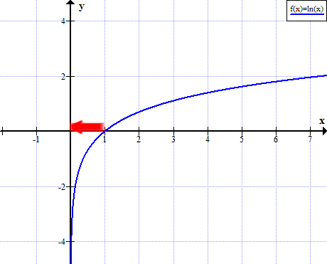
   Figure 5: LogX becomes large when X reaches to zero

   
   

   Inference Process: the model will predict the first word, which then is fed back into the model to predict the next word. This process continues until the prediction is complete.

   
   
   

5. Reinforcement Learning (RL) :
   • Definition: Reinforcement Learning (RL) is a separate approach in Machine Learning that focuses on training models through interactions with an environment, rather than just learning from existing data (like supervised or unsupervised learning).
   • Complexity: RL is conceptually and mathematically challenging.
   • Niche Applications: While powerful, its applications (e.g., robotics, game AI) are narrower compared to others.
   • Techniques: Markov Decision Processes, policies, rewards, and exploration/exploitation trade-offs.

   
   
   

   

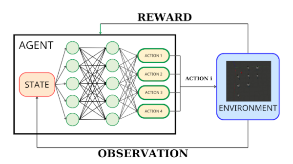
   Figure 5: Reinforcement Learning

   Let’s attach this diagram to a real case to get to understand an RL. Imagine we train a agent (model) for steering a car automatically. We want to go from point A to point B. Now there are 2 tasks to do:

   • Task 1 : Set the map from A to B with the possible shortest distance and a clear fee.
   • Task 2 : Drive the car when there are many other obstacles on the street like pedestrians, other cars, crossroads lights, or even cats. In fact, it also needs to drive under traffic law like a real human, following instructions of traffic signals in the street.

   And here Reinforcement Learning is trained to handle only the task 2:

   • Agent : a neural network recieves a state $s_{t}$ (obstacles, traffic signals) from the environment at time $t$.

   • Action $a_{t}$ : (turn right or left, slow down, speed up, or brake) Based on $s_{t}$, the agent produces an antion $a_{t}$ via the network models, this means there are more than one type of Reinforcement Learning.

   • Reward $r_{t}$ : a immediate reward (how many points) recieved after action $a_{t}$ is applied to the environment, then the system comes to a new state $s_{t+1}$. Reward for each action is set manually based on context. For driving a car, how many points to avoid pedestrians by either turning left or turning right or slowing down or just keep the current state, how many points to achieve a speed that is either energy-saving or legal or comfortable.

   • Policy ($\pi$) : a strategy the agent follows to find and take the best action, denoted $\pi(a_{t} | s_{t})$, implying the probability of taking action $a_{t}$ in state $s_{t}$. Each policy will have different settings of rewarding, meaning reward of one action will change under different policies. Particularly, for driving a car, we have several policies: “normal driving”, “night driving”, “snow driving” and etc. Action “passing another car” will get sure “smaller reward points” under “snow driving” policy and “higher reward points” under “normal driving” policy.

   • Discount factor ($\gamma$) : between [0,1] that implies the important degree of future rewards, controlling the trade-off (sự đánh đổi) between immediate and future rewards.

   • 1. What is the Goal here in Reinforcement Learning : Find the optimal policy $\pi^{*}$ that could maximize the expected cumulative reward or the total rewards starting from time step t:
   \[G_{t} = \sum_{k=0}^{\infty} \gamma_{k} \cdot r_{t+k+1}\]
   • 2. The Bellman equation : It is central in Reinforcement Learning and a mathematical way to define the relationship between a state and its expected reward over time, helping the agent make decisions based on the maximum value $V(s)$:
   \[V(s) = \underset{a}{max} \Bigr[r(s,a) + \gamma \cdot \sum_{s'}P(s'|s,a) \cdot V(s') \Bigr]\]

   With:

   • $P(s’ | s, a)$ is the probability of transitioning to a new state $s’$ from $s$ after taking an “perfect” action $a$.
   • $V(s’)$ is value from new state $s’$.

   Explaination: in most cases, from state $s$, there will be more than one new state $s’$ to select and because different $s’$ will give different rewards, the agent has to learn to choose the one with highest $V(s)$.

   From here, Apply Bellman into the $V and \ Q$ equations in the Reinforcement Learning under a specific policy $\pi$, we can decompose the value functions recursively:

   \[V^{\pi}(s) = \sum_{a \in A} \pi(a|s) \sum_{s' \in S} P(s'|s, a) \Bigr[r(s,a) + \gamma \cdot V^{\pi}(s') \Bigr]\] \[Q^{\pi}(s,a) = \sum_{s' \in S}P(s'|s, a) \cdot \Bigr[r(s,a) + \gamma \cdot \sum_{a' \in A} \pi(a',s')Q^{\pi}(s',a') \Bigr]\]
   • The relationship between $V and \ Q$ : It is easy to see that $Q$ is calculated based on a specific action, while $V$ is based only on stateful transitions. Hence, for a specific state, $\ V$ is the maximum value over all possible actions $a$ in $Q(s,a)$ at this state.
   \[V(s) = \underset{a}{max}Q(s,a)\]

   For an optimal policy $\pi^{*}$ :

   \[V^{*}(s) = \underset{a \in A}{max} \sum_{s' \in S} P(s'|s, a) \Bigr[r(s,a) + \gamma \cdot V^{*}(s') \Bigr]\] \[Q^{*}(s,a) = \sum_{s' \in S}P(s'|s, a) \cdot \Bigr[r(s,a) + \gamma \cdot \underset{a \in A}{max} Q^{*}(s',a') \Bigr]\]

   Although, Bellman equation is the key of RL, there are still many “learning approaches” to build a RL model: “model-based methods” or “model-free methods”.

   • Remark: what is model-based and model-free models?
   • Firstly, the word “model” used here is ir-relevant to the neuron network in AI. Here, the model is the model of environment.
   • Model-based models: It needs a model of environment, where everything is predictable or next states can be predicted. It’s like playing a chess, the agent tries to predict as many as possible states or opponents possible moves to make a next move. Here, the computation of prediction is expensive.
   • Model-free models: There’s no a model of environment, the agent uses experience to interact directly with the environment. It estimates the “rewards” of actions or states to decide what to do instead of prediction. It’s like a robot dog which you can put in a park, a house or in the streets. The “dog” will take action directly based on the environment by what it has been trained.

   Back to this post, I will mention 2 common model-free approaches: TD Learning and Q-Learning:
   

   A. Temporal-Difference (TD) Learning :

   • A.1 Core Idea : In TD-Learning, the value function $V$ is updated based on the difference between the current value estimate and a “better” estimate formed using observed rewards and the value of the next state.

   • For a given policy $\pi$ with an input data of states coupled with specific rewards, at current state $s_{t}$, TD-Learning will approximates $V$ iteratively for each possible next states. (of course, there’s only one target state among these states):

   \[V^{\pi}(s) = \mathbb E_{\pi} \Bigr[ \sum_{k=0}^{\infty} \gamma_{k} \cdot r_{t+k+1} | s_{t}=s \Bigr]\]

   
   

   • A.2 Error or Loss : The TD error ($\delta$, “delta”) quantifies the difference between the current value estimate and a one-step lookahead estimate:
   \[\delta_{t} = r_{t+1} + \gamma V(s_{t+1}) - V(s_{t})\]

   With:

   • $r_{t+1}$ is the immediate reward as transitioning from $s_{t}$ to $s_{t+1}$,
   • $V(s_{t})$ is the current value estimate of state $s_{t}$,
   • $V(s_{t+1})$ is the current value estimate of state $s_{t+1}$,

   The loss function for TD learning is usually the Mean Squared Error (MSE) of the TD error:

   \[Loss = \frac{1}{2} \delta^{2} = \frac{1}{2} (r_{t+1} + \gamma V(s_{t+1}) - V(s_{t}))^{2}\]

   So

   \[\frac{\partial Loss}{\partial V(s)} = \frac{\partial}{\partial V(s)} (\frac{1}{2} \delta^{2}) = \delta \cdot \frac{\partial \delta}{\partial V(s)} = -\delta\]

   
   

   • A.3 Update Rule : The value V is updated incrementally with learning rate $\alpha$:
   \[V(s_{t}) \leftarrow V(s_{t}) + \alpha \delta_{t}\]

   Replace $\delta$ into the update rule:

   \[V(s_{t}) \leftarrow V(s_{t}) + \alpha \Bigg( r_{t+1} + \gamma V(s_{t+1}) - V(s_{t}) \Bigg)\]
   • A.4 With Weight matrix (W):
   \[V(s) = W \cdot \phi(s)\]

   With:

   • $W$ is the weight matrix that need to be learned,
   • $\phi(s)$ is the input data of states. (For ex: the distance to obstacles,…)

   And the learning gradient equation:

   \[W \leftarrow W - \alpha \cdot \frac{\partial Loss}{dW}\] \[W \leftarrow W - \alpha \cdot \frac{\partial Loss}{dV} \cdot \frac{\partial V}{\partial W} = W + \alpha \cdot \delta \cdot \frac{\partial V}{\partial W}\] \[W \leftarrow W + \alpha \cdot \Big( r_{t+1} + \gamma V(s_{t+1}) - V(s_{t}) \Big) \cdot \phi(s_{t})\]
   B. Deep Q-Learning :

   Deep Q-Learning (DQN) is an extension of Q-Learning where a deep neural network is used to approximate the Q-value function. The neural network’s weight matrix W to learn a mapping from states s (or state-action pairs) to their corresponding Q-values.

   B.1 Initialization:

   • Neural network weights $W$ with random values.
   • Target network weights $W^{-}$, initially set to $W$.

   B.2 For each episode:

   • Step 1: start in state $s$.
   • Step 2: Choose an action $a$ using an exploration policy (e.g greedy policy = max immediate reward).
   • Step 3: Take action $a$, observe reward $r$ and next state $s’$.
   • Step 4: Store (past) transition ($s,a,r,s’$) in the replay buffer $D$.
   • Step 5: Sample a mini-batch of transitions from the buffer $D$.
   • Step 6: Compute the target Q-value $y$ for each transition using the target network $W^{-}$.
   \[y = r + \gamma \cdot \underset{a'}{max} Q(s',a'; W^{-})\]

   With $Q(s’,a’;W^{-})$ represents the target Q-value of the next state $s’$ and action $a’$.

   Why Use the Target Network? :

   If we use the same network $W$ to computes both the current and target $Q-values$, it can lead to instability. This happens because the targets themselves are changing as the network learns, causing feedback loops and divergence(phân kỳ).

   The target network solves this problem by keeping the target $Q(s’,a’;W^{-})$ relatively stable during training. The weights of the target network $W^{-}$ are only updated periodically, rather than after every training step.

   • Step 7: Compute the Loss $L(W)$ following the Mean Squared Error between the predicted and target Q:
   \[L(W) = \mathbb E_{s,a,r,s'} \bigr[ \big( \ y - Q(s,a; W) \ \big)^{2} \bigr]\]
   • Step 8: Perform a gradient descent step to update W. The weights $W$ are updated using stochastic gradient descent (SGD):
   \[W \leftarrow W + \alpha \cdot \Delta_{W}L(W)\] \[\Delta_{W}L(W) = -2 \big( y-Q(s,a;W) \cdot \Delta_{W}Q(s,a;W) \big)\]

   $\Delta_{W}Q(s,a;W) = \frac{\partial Q}{\partial W}$ : The derivative of the predicted Q-value with respect to the weights

   • Step 9: Periodically update $W^{-}$ with $W$ (e.g. every N steps).

   B.3 End When Converged.

   B.4 Summary : Mathematically, the key steps involve computing the target $y$, minimizing the loss $L(W)$, and updating $W$ via backpropagation.
   
   

6. Graph Neural Networks (GNNs) :
   • GNN is designed to work directly on graph-structured data. Graphs consist of nodes (vertices) and edges, making them ideal for representing relationships between entities, such as social networks, molecules, transportation networks, or recommendation systems.
   • Graphs: have a non-Euclidean structure, meaning they don’t fit neatly into grids or sequences.
   • GNNs overcome this limitation by learning to represent and process data with irregular connections and relationships.
     
     
   

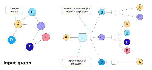
   Figure 6: Graph Neural Networks (GNNs)

Additional Recommendations :

• For interests in generative AI, such as creating images or videos, consider Generative Adversarial Networks (GANs) after mastering CNNs.
• If you’re working with low data, delve into Few-Shot Learning Models.