
An LLM (Large Language Model) is a programming function that specializes in processing, understanding, and generating human-like text, performing tasks like language translation, code generation and completion, text generation, text classification, and question-answering,… .
This post will dig into the core building blocks of LLMs, focusing on transformer architectures and the latest models Gemini of Google.
-
Types of Large Language Model Architechture:
-
RNNs (Recurrent neuron networks): RNNs process input and output sequences sequentially. They generate a sequence of hidden states based on the previous hidden state and the current input, making them hard to parallelize during training.
-
Transformer: it can process sequences of tokens in parallel thanks to the self-attention mechanism. This results in faster training. However, the cost of self-attention is quadratic in the context length which limits the size of the context, while RNNs have a theoretically infinite context length.
-
-
the first version of Transformer: Translation Model
- Its architecture consists of two parts: an encoder and a decoder. The encoder converts the input text (a French sentence) into a representation, which is then passed to the decoder. The decoder uses this representation to generate the output text (an English translation). Notably, the size of the output of the transformer encoder is linear in the size of its input.
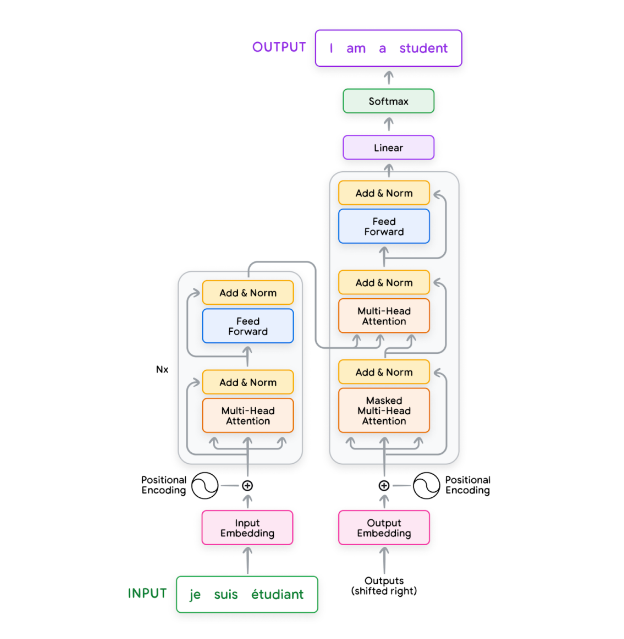
Figure 1: Original Transformer
- To better understand the different layers in the transformer, we will also describe each of the components inside the Figure 1.
- Input embedding (preparation): text input => vectors (input embedding)
- Normalization (Optional) : removing redundant whitespace, accents, etc.
- Tokenization : Breaks the sentence into words or subwords and maps them to integer token IDs from a vocabulary.
- Embedding : Converts each token ID to its corresponding high-dimensional vector, typically using a lookup table.
- Positional Encoding : Adds information about the position of each token in the sequence to help the transformer understand word order.
-
Multi-head attention : “Self-attention” is a crucial mechanism in this step. It helps to determine relationships between different words and phrases in a text input. Consider the sentence: “The tiger jumped out of a tree to get a drink because it was thirsty.” In this sentence, “the tiger” and “it” are the same object, so we would expect these 2 words to be strongly connected.
2.1 Creating queries (Q), keys (K), and values (V): each input embedding is multiplied by three learned weight matrices Wq, Wk, Wv to generate 3 vectors Q, K and V:
- Q (which word?): helps the model ask, “Which other words in the sequence are relevant to me?”
- K (how relevant?): like a label that helps the model identify how a word might be relevant to other words in the sequence.
- V (actual meaning): holds the actual word content information.
2.2 Scores : Scores determine how much each word should ‘attend’ to other words. This is done by taking the dot product of the query vector (Q) of one word with the K vectors of all the words in the sequence.
2.3 Normalization: The scores are divided by the square root of the key vector dimension (dk) for stability, then passed through a softmax function to obtain attention weights. These weights indicate how strongly each word is connected to the others.
-
$d_{k}$ is the dimension of the query and key vectors. If the model dimentionality $𝑑_{model}$ = 512 and the config has 8 attention heads, each head will usually have a key dimension $d_{k}$ = 512/8 = 64.
-
In NLP, the model dimensionality is the length of word embeddings.
2.4 Weighted values: Each value vector is multiplied by its corresponding attention weight. The results are summed up, producing a context-aware representation for each word.
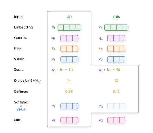
Figure 2: "Self attention" computation process
- The dimensionality of embeddings
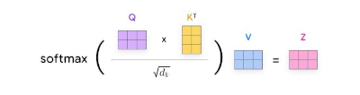
Figure 2: the basic of self attention calculation
-
Power in diversity of Multi-head attention: There are 8 heads with its own Q, K and V, each ‘head’ potentially focusing on different aspects of the input relationships. Each head calculates its own attention scores. The output of each head is concatenated to form a single vector Z, which is then linearly transformed back to the original model dimension $d_{model}$. This helps:
- Handle complex language patterns and long-range input.
- The calculations of each head can run in parallel.
- Layer normalization and residual connections (unclear): Each layer in a transformer, consisting of a multi-head attention module and a feed-forward layer, employs layer normalization and residual connections.
- Layer normalization computes the mean and variance of the activations to normalize the activations in a given layer.
-
Feedforward layer (unclear): The feedforward layer typically consists of two linear transformations with a non-linear activation function, such as ReLU or GELU, in between.
-
Encoder and decoder (unclear):
-
The original transformer architecture relies on a combination of encoder and decoder modules. Each encoder and decoder consists of a series of layers, with each layer comprising key components: a multi-head self-attention mechanism, a position-wise feed-forward network, normalization layers, and residual connections.
-
The encoder’s primary function is to process the input sequence into a continuous representation that holds contextual information for each token. The input sequence is first normalized, tokenized, and converted into embeddings. Positional encodings are added to these embeddings to retain sequence order information. Through self-attention mechanisms, each token in the sequence can dynamically attend to any other token, thus understanding the contextual relationships within the sequence. The output from the encoder is a series of embedding vectors Z representing the entire input sequence.
-
The decoder (unclear) is tasked with generating an output sequence based on the context provided by the encoder’s output Z. It operates in a token-by-token fashion, beginning with a start-of-sequence token. The decoder layers employ two types of attention mechanisms: masked self-attention and encoder-decoder cross-attention.
- Masked self-attention ensures that each position can only attend to earlier positions in the output sequence, preserving the auto-regressive property. This is crucial for preventing the decoder from having access to future tokens in the output sequence.
- The encoder-decoder cross-attention mechanism allows the decoder to focus on relevant parts of the input sequence, utilizing the contextual embeddings generated by the encoder. This iterative process continues until the decoder predicts an end-of-sequence token, thereby completing the output sequence generation.
-
- Training: In machine learning models, it’s important to differentiate between training and inference.
- Training typically refers to modifying the parameters of the model, and involves loss functions and backpropagation.
- Inference is when model is used only for the predicted output, without updating the model weights.
-
Data preparation : involves a few important steps:
- Clean the data by applying techniques such as filtering, deduplication, and normalization.
- Tokenization where the dataset is converted into tokens using techniques such as Byte-Pair Encoding and Unigram tokenization. Tokenization generates a vocabulary, which is a set of unique tokens used by the LLM. This vocabulary serves as the model’s ’language’ for processing and understanding text.
- Finally, the data is split into a training dataset for training the model as well as a test dataset which is used to evaluate the models performance.
-
Loss function : a typical transformer training loop consists of several parts:
- Batches: batches of input sequences are sampled from a training dataset. For each input sequence X, there is a corresponding target sequence $Y_{target}$. In unsupervised pre-training, the target sequence is derived from the input sequence itself.
- Loss Function: the difference between the predicted and target sequences is measured using a loss function (often cross-entropy loss). Gradients of this loss are calculated, and an optimizer uses them to update the transformer’s parameters (W).
Training Task: There are different approaches depending on the architecture used:
9.1 Decoder-only models : The target sequence for the decoder is simply a shifted version of the input sequence. Given a training sequence like ‘the cat sat on the mat’ various input/target pairs can be generated for the model.
For example the input “the cat sat on” should predict “the” and subsequently the input “the cat sat on the” should predict target sequence “mat”.9.2 Encoder-only models (like BERT) are often pre-trained by corrupting the input sequence in some way and having the model try to reconstruct it. One such approach is masked language modeling (MLM). In our example, the input sequence could be “The [MASK] sat on the mat” and the sequence target would be the original sentence.
9.3 Encoder-decoder models (like the original transformer) are trained on sequence-to-sequence supervised tasks such as translation (input sequence “Le chat est assis sur le tapis” and target “The cat sat on the mat”), question-answering (where the input sequence is a question and the target sequence is the corresponding answer), and summarization (where the input sequence is a full article and the target sequence is its corresponding summary). These models could also be trained in an unsupervised way by converting other tasks into sequence-to-sequence format. For example, when training on Wikipedia data, the input sequence might be the first part of an article, and the target sequence comprises the remainder of the article.
-
Popular models:
-
GPT-3: GPT-3 stands for Generative Pre-trained Transformer model with 175 billion parameters. GPT-3 exhibits improved performance from translation to question-answering. GPT-3.5 is capable of understanding and generating code.
-
GPT-4 extends GPT-3.5 as a large multimodal model capable of processing image and text inputs and producing text outputs. Specifically, accepting text or images as input and outputting text. It can receive context windows of up to 128,000 tokens and has a maximum output of 4,096 tokens.
-
Gemini can receive multi-modal inputs including text, audio, images, and video data. The output can contain images and text. In 2024, Google introduced the latest model of the Gemini family, Gemini 1.5 Pro. It can functions: code understanding, language learning (The model can learn new languages provided within its input), video comprehension: (It can analyze entire movies, answering detailed questions and pinpointing specific timestamps).
-
-
Fine Tuning: Large language models typically undergo multiple training stages:
-
Pre-training, is the foundational stage where an LLM is trained on large, diverse, and unlabelled text datasets where it’s tasked to predict the next token given the previous context. The goal of this stage is to leverage a large, general distribution of data and to create a model that is good at sampling from this general distribution. Pretraining is the most expensive in terms of time (from weeks to months depending on the size of the model) and the amount of required computational resources, (GPU/TPU hours).
-
Fine Tune (SFT): After pre-training, the model can be further specialized via fine-tuning. SFT is the process of improving an LLM’s performance on a specific task or set of tasks by further training it on domain-specific, labeled data. The dataset is typically significantly smaller than the pre-training datasets, and is usually human-curated and of high quality.
- Each data point consists of an input (prompt) and a demonstration (target response). For example, questions (prompt) and answers (target response), translations from to another language (target response), a document to summarize (prompt), and the corresponding summary (target response).
-
Reinforcement learning from human feedback (RLHF) : Typically, after performing SFT, a second stage of fine-tuning occurs which is called reinforcement learning from human feedback (RLHF). This enables an LLM to better align with human-preferred responses.
- In contrast to SFT, where an LLM is only exposed to positive examples (e.g. high-quality demonstration data), RLHF makes it possible to also leverage negative outputs thus penalizing an LLM when it generates responses that exhibit undesired properties.
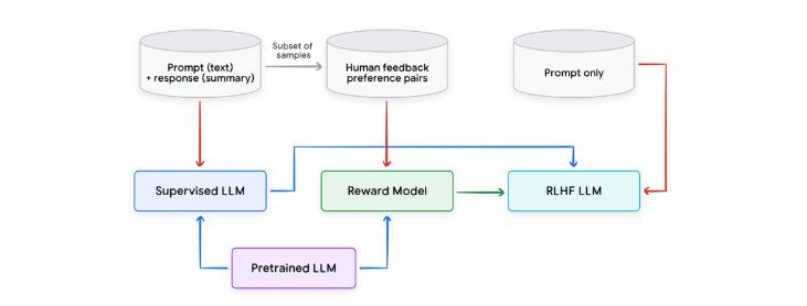
Figure 7: RLHF
- To leverage RLHF, a reward model (RM) typically needs to be trained with a procedure similar to that in Figure 7. An RM is usually initialized with a pretrained transformer model. Then it is tuned on human preference data which is either single sided (with a prompt, response and a score) or composed of a prompt and a pair of responses along with a preference label indicating which of the two responses was preferred. For example, given two summaries, A and B, of the same article, a human rater selects a preferred summary (relying on the detailed guidance). The preference signal can also incorporate many dimensions that capture various aspects that define a high quality response, e.g., as safety, helpfulness, fairness, and truthfulness.
-
-
Parameter Efficient Fine-Tuning (PEFT) : PEFT can make fine-tuning significantly cheaper and faster compared to pre-training and full fine-tuning. Some common PEFT techniques:
-
Adapter-based fine-tuning employs small modules, called adapters, to the pre-trained model. Only the adapter parameters are trained, resulting in significantly fewer parameters than traditional SFT.
-
Low-Rank Adaptation (LoRA) tackles differently. It uses two smaller matrices to approximate the original weight matrix update instead of fine-tuning the whole LLM. This technique freezes the original weights and trains these update matrices, significantly reducing resource requirements with minimum additional inference latency. A nice advantage of LoRA modules is that they can be plug-and-play, meaning you can train a LoRA module that specializes in one task and easily replace it with another LoRA module trained on a different task. It also makes it easier to transfer the model.
-
Soft prompting (unclear):
-